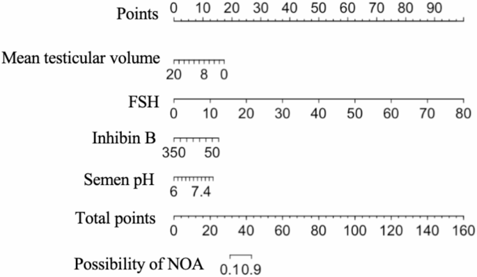
Developing a nomogram model for predicting non-obstructive azoospermia using machine learning techniques

Study population and observational index

A retrospective study was conducted on 352 patients diagnosed with azoospermia, collected by the Department of Andrology and Sexual Medicine of the First Affiliated Hospital of Fujian Medical University from January 2020 to February 2024. This study received approval from the Medical Ethics Committee of the First Affiliated Hospital of Fujian Medical University (MRCTA, ECFAH of FMU [2019] 213 and [2020] 375) and was conducted in compliance with the principles outlined in the Declaration of Helsinki. Informed written consent was obtained from all participants.

Azoospermia was confirmed in all patients after more than three semen centrifugation procedures (3000 g, 15 min; Centrifuge 5425, Eppendorf, Hamburg, Germany) spaced over two week intervals, yielding no detectable sperm¹³. The exclusion criteria included patients with hypogonadotropic hypogonadism, individuals under 14 years old, and those with incomplete clinical data. Detailed medical histories were obtained, including inquiries about orchitis, epididymitis, mumps, prior testicular trauma and surgery, and cryptorchidism status. Similarly, potential iatrogenic causes, such as the use of gonadotoxic medications, prior radiation exposure, and environmental exposure, were all taken into consideration. Patients with cryptorchidism had undergone orchiopexy at least six months prior to the study.

Testicular volume (TV) was determined using using a Prader’s orchidometer by two experienced andrologists (Song-xi Tang and Hui-liang Zhou). Subsequently, the volumes of the left and right testes were summed and averaged to calculate the mean testicular volume (MTV) for each patient. Ejaculate volume and semen pH were averaged from multiple assessments. The clinical assessments included measuring serum levels of prolactin, follicle-stimulating hormone (FSH), luteinizing hormone (LH), estradiol, testosterone (T), and inhibin B (INHB) between 8:00 a.m. and 10:00 a.m. Varicocele was diagnosed through physical examination conducted by two seasoned andrologists (Hui-liang Zhou, and Song-xi Tang) in conjunction with color Doppler ultrasound.

Patients initially diagnosed with NOA must undergo karyotype analysis of peripheral blood and Y chromosome microdeletion analyses; whole-exome sequencing is deemed unnecessary. Patients being assessed for OA underwent evaluations utilizing color Doppler ultrasound (GE LOGIQ Fortis, GE Healthcare, Chicago, USA) or magnetic resonance imaging (Magnetom Prisma, Siemens, Munich, Germany) along with physical examinations to determine the site of obstruction.

Histopathological analysis of the testis.

Histopathological examination of the testis involved embedding the testicular tissues in paraffin and serially sectioning them at a thickness of 4 μm for routine hematoxylin and eosin staining. The sections were observed under light microscopy (CKX31, Olympus, Tokyo, Japan). The condition characterized by the presence of only Sertoli cells was classified as SCOS. Maturation arrest (MA) was diagnosed when spermatogonia, primary spermatocytes, secondary spermatocytes, or spermatids were present without mature sperm. Hypospermatogenesis referred to testicular pathology where a small amount of mature sperm was observable. Diagnosis was based on the predominant histopathological pattern observed. Patients with testicular pathological conditions such as SCOS, MA, or hypospermatogenesis were classified as NOA, whereas specimens exhibiting normal or near-normal spermatogenesis were classified as OA¹⁴.

Statistical analysis

Statistical analysis was performed using SPSS software version 27.0 (IBM Corp., Armonk, NY, USA). Continuous variables were expressed as means ± standard deviation or medians with interquartile ranges, while categorical variables were presented as frequencies or percentages. The Shapiro-Wilk test was used to assess data distribution, and Levene’s test evaluated variance homogeneity. Non-normally distributed continuous variables were compared using the U-test. The application of Pearson’s chi-square and Fisher’s exact probability tests were utilized to compare rates between groups. Univariate and multivariate logistic regression analyses were conducted to identify independent risk factors. From the entire dataset, 70% was randomly selected for training the models, while the remaining 30% was allocated for testing.

The machine learning algorithms and nomogram was constructed within R version 4.2.3 (R Foundation for Statistical Computing, Vienna, Austria). We utilized nine distinct machine learning algorithms for modeling: Random Forest, Gradient Boosting Decision Trees (GBDT), XGBoost, LightGBM, Naive Bayes, Support Vector Machine (SVM), Logistic Regression, Decision Trees, and Neural Networks. The Random Forest model ensures reproducibility by optimizing the “mtry” hyperparameter using “tuneRF” and applying regularization through parameters such as “ntree = 500,” “nodesize = 5,” and “maxnodes = 30” to mitigate overfitting and enhance stability. The GBDT model optimizes hyperparameters via 5-fold cross-validation, tuning key parameters including “n.trees = 100,” “interaction.depth = 3,” “shrinkage = 0.05,” and “n.minobsinnode = 10” to balance complexity and reduce overfitting. Similarly, the XGBoost model employs 5-fold cross-validation with early stopping to mitigate overfitting. Parameters such as “max_depth = 6,” “eta = 0.1,” “subsample = 0.8,” “colsample_bytree = 0.8,” “min_child_weight = 1,” “lambda = 1,” and “alpha = 0” are tuned to manage complexity, with the optimal number of boosting rounds determined to ensure reproducibility. The LightGBM model follows a similar approach, using 5-fold cross-validation and early stopping (limited to 10 rounds) to prevent overfitting. Parameters such as “num_leaves = 31,” “learning_rate = 0.05,” “feature_fraction = 0.8,” “bagging_fraction = 0.8,” “bagging_freq = 5,” “lambda_l1 = 0.1,” “lambda_l2 = 0.1,” and “min_data_in_leaf = 20” are selected to balance model complexity and reproducibility by determining the optimal number of boosting rounds. The Naive Bayes model is trained using 5-fold cross-validation, with hyperparameter tuning on the Laplace smoothing parameter (“laplace = 0, 0.5, 1”), kernel usage, and the adjustment factor (“adjust = 1”), ensuring reproducibility with consistent tuning parameters and cross-validation settings. The SVM model uses a radial basis function kernel, tuning hyperparameters such as “C” (cost) and “sigma” (gamma) through 5-fold cross-validation and grid search (“C = 0.1, 1, 10” and “sigma = 0.01, 0.05, 0.1”) to prevent overfitting and ensure reproducibility. The Logistic Regression classifier employs Lasso regularization (“alpha = 1”) and is trained via 5-fold cross-validation (“nfolds = 5”) to select the optimal regularization parameter (“lambda.min”), promoting model generalization and preventing overfitting through automatic hyperparameter tuning. Reproducible results are achieved based on a fixed dataset and consistent parameter settings. The Decision Tree model is tuned through 10-fold cross-validation, adjusting parameters such as “cp = 0.01,” “minsplit = 20,” and “maxdepth = 5” to prevent overfitting and ensure reproducibility by controlling complexity and optimizing generalization. Finally, the Neural Network model uses 10-fold cross-validation, tuning hyperparameters such as the number of hidden units (“size = 5, 10, 15”) and regularization strength (“decay = 0, 0.001, 0.01”) to prevent overfitting with L2 regularization, ensuring reproducibility through consistent parameter settings and cross-validation.

The predictive performance was assessed using the area under the receiver operating characteristic (ROC) curve. Graphs were created using GraphPad Prism 10.0 (GraphPad Software Inc., San Diego, CA, USA). The calibration curve and decision curve analysis (DCA) were calculated using R software. Statistical significance was set at P < 0.05 for all two-tailed tests.