The risk factors determined by four machine learning methods for the change of difference of bone mineral density in post-menopausal women after three years follow-up

Participant and study design
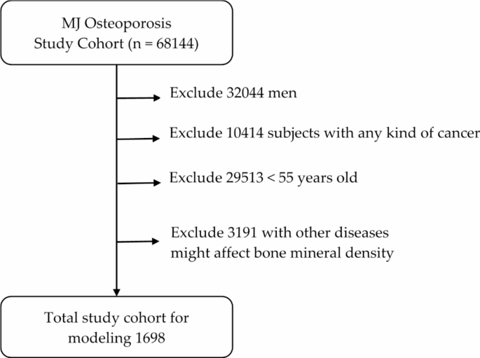
The data for this study were obtained from the Taiwan MJ cohort, an ongoing prospective cohort of health examinations conducted by the MJ Health Screening Centers in Taiwan10,11,12,13,14. These comprehensive examinations cover more than 100 essential biological indicators, including anthropometric measurements, blood tests, and imaging tests, among others. Additionally, each participant completed a self-administered questionnaire to provide information on personal and family medical history, current health status, lifestyle, physical exercise, sleep habits, and dietary habits10,11,12,13,14,15. Only participants who provided informed consent were included in the MJ Health Database, and the study protocol was approved by Institutional Review Board of the Kaohsiung Armed Forces General Hospital (IRB No.: KAFGHIRB 109 − 041). The description of the cohort was published by our group previously16. In the present study, all methods were performed in accordance with the relevant guidelines and regulations of our institution. A total of 3,412 healthy women aged 55 years and above were initially enrolled, and after excluding subjects with various causes, 1,698 subjects remained for analysis, as depicted in Fig. 1. The data that support the findings of this study are available from MJ clinic but restrictions apply to the availability of these data, which were used under license for the current study, and so are not publicly available. Data are however available from the corresponding author upon reasonable request and with permission of MJ clinic.

Patient selection scheme.
On the day of the study, senior nursing staff recorded each subject’s medical history, including information on any current medications, and performed a physical examination. The waist circumference was measured horizontally at the level of the natural waist, and the body mass index (BMI) was calculated as the participant’s body weight (kg) divided by the square of their height (m). The systolic blood pressure (SBP) and diastolic blood pressure (DBP) were measured using standard mercury sphygmomanometers on the right arm of each subject while seated.
The procedures for collecting demographic and biochemical data were consistent with previously published methods13. After fasting for 10 h, blood samples were collected for biochemical analyses. Plasma was separated from the blood within 1 h of collection and stored at 30 °C until the analysis of fasting plasma glucose (FPG) and lipid profiles. FPG was measured using the glucose oxidase method (YSI 203 glucose analyzer; Yellow Springs Instruments, Yellow Springs, OH, USA). The total cholesterol and triglyceride (TG) levels were measured using the dry multilayer analytical slide method with a Fuji Dri-Chem 3000 analyzer (Fuji Photo Film, Tokyo, Japan). The serum high-density lipoprotein cholesterol (HDL-C) and low-density lipoprotein cholesterol (LDL-C) concentrations were analyzed using an enzymatic cholesterol assay, following dextran sulfate precipitation. Additionally, the urine albumin-to-creatinine ratio (ACR) was determined by turbidimetry using a Beckman Coulter AU 5800 biochemical analyzer. The T score was measured by dual-energy X-ray absorptiometry (Lunar, General Electric Company, USA).
Traditional statistics
The data are presented as means ± standard deviations. To assess the differences in continuous data between men and women, the Student t-test was employed. Additionally, the relationships between δ-T score and all other variables were analyzed using Pearson’s correlation. All statistical tests were two-sided, and a p-value less than 0.05 was considered statistically significant. The statistical analysis was conducted using SPSS 10.0 for Windows (SPSS, Chicago, IL, USA).
Proposed machine learning scheme
This study proposes a scheme based on four different Machine Learning (Mach-L) methods, namely, Random Forest (RF), eXtreme Gradient Boosting (XGBoost), Naïve Bayes (NB), and stochastic gradient boosting (SGB), to construct predictive models for δ-BMD after a four-year follow-up. These Mach-L methods have been widely applied in various healthcare applications and do not rely on prior assumptions regarding data distribution14,15,17,18,19,20,21,22,23,24. This part of method has been published by our group25.
Random Forest (RF) is an ensemble learning decision trees algorithm that combines bootstrap resampling and bagging26. Its principle involves randomly generating multiple different and unpruned CART decision trees, where the decrease in Gini impurity is used as the splitting criterion. All the generated trees are then combined to form a forest. The final model is obtained by averaging or voting among all the trees in the forest to generate output probabilities and ensure robustness27.
The next method, SGB, is a tree-based gradient boosting learning algorithm that combines bagging and boosting techniques to minimize the loss function and address the over-fitting problem of traditional decision trees28,29,30. In the SGB, it sequentially generates many stochastic weak learners (trees) through multiple iterations. Each tree focuses on correcting or explaining errors from the tree of the previous iteration, with the residual of the previous iteration tree serving as the input for the newly generated tree. This iterative process continues until a stopping criterion is reached, such as the maximum number of iterations or the convergence condition. Ultimately, the cumulative results of many trees are used to determine the final robust model.
The third method is NB, a popular Mach-L model used for classification tasks. This algorithm can sort objects based on specific characteristics and variables, using the Bayes theorem to calculate the probability of hypotheses on presumed groups31. Unlike logistic regression, Mach-L methods like NB do not require strong model assumptions and are capable of capturing delicate underlying nonlinear relationships present in empirical data14.
As for XGBoost, it is the final method utilized in this study, and it is a gradient boosting technology based on the optimized extension of SGB32. The underlying principle of XGBoost involves training many weak models sequentially and assembling them using the gradient boosting method to achieve improved prediction performance. To accelerate the model construction convergence process, XGBoost employs the Taylor binomial expansion to approximate the objective function and utilizes arbitrary differentiable loss functions33. Additionally, XGBoost applies a regularized boosting technique to penalize the complexity of the model, thereby correcting overfitting and increasing model accuracy32.
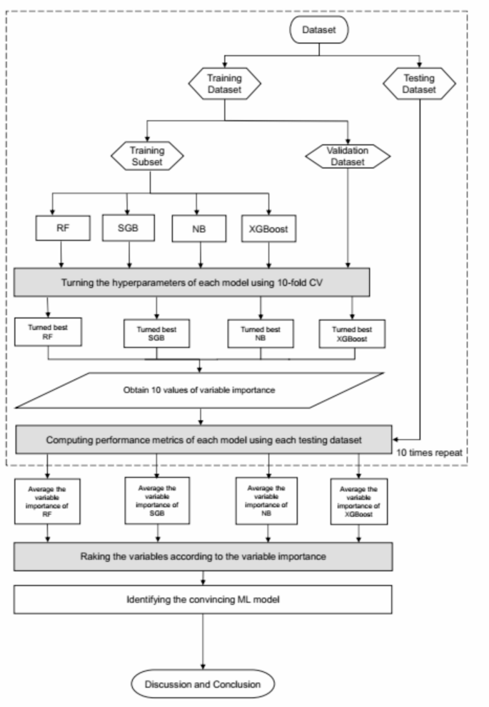
Figure 2 presents the flowchart of the proposed prediction and important variable identification scheme that combines the four Mach-L methods. Initially, patient data were collected and used to prepare the dataset through the proposed method. Subsequently, the dataset was randomly divided into an 80% training dataset for model building and a 20% testing dataset for model evaluation. During the training process, each Mach-L method was fine-tuned with specific hyperparameters to construct well-performing models. To achieve this, a 10-fold cross-validation (CV) technique was employed for hyperparameter tuning. The training dataset was further partitioned into a training subset with a different set of hyperparameters and a validation subset for model validation. A grid search explored all possible combinations of hyperparameters. The model with the lowest root mean square error for the validation subset was deemed the best model for each ML method. Consequently, the best-tuned RF, SGB, NB, and XGBoost models were generated, and the corresponding variable importance ranking information was obtained.

Proposed machine learning prediction scheme.
For the testing process, the testing dataset was utilized to assess the predictive performance of the best RF, SGB, NB, and XGBoost models. Since the target variable in this study is a numerical variable, model performance comparison utilized metrics such as the symmetric mean absolute percentage error (SMAPE), relative absolute error (RAE), root relative squared error (RRSE), and root mean squared error (RMSE), which are presented in Table 1. SMAPE is a useful, balanced way to verify the mean percentage of error for predicted results. The basal MAPE formula places only the absolute value of the actual value into the denominator, which gives the restriction that no instance may be the actual value is zero or very small. As an alternative, SMAPE was used. The RAE is calculated as the sum of the absolute differences between the predicted and actual values, divided by the sum of the absolute differences between the actual values and the mean of the actual values. This metric provides an intuitive way to assess the accuracy of a model in relation to a simple baseline, making it useful for comparing different predicted methods. RMSE is calculated as the square root of the average of the squared differences between the predicted and actual values, RMSE penalizes larger errors more heavily, making it sensitive to outliers and providing a clear indication of the model’s accuracy. RRSE is determined by dividing the sum of the squared differences between the predicted and actual values by the sum of the squared differences between the actual values and the mean of the actual values, and then taking the square root of the result. The SMAPE, RAE, RRSE, and RMSE are lower values that indicate better prediction, as it signifies that the model’s prediction values are closer to the actual values.
To ensure a robust comparison, the training and testing processes mentioned above were repeated randomly for 10 iterations. The averaged metrics of the RF, SGB, NB, and XGBoost models were then utilized to compare the model performance against the benchmark MLR model, which used the same training and testing datasets as the Mach-L methods. A Mach-L model with an average metric lower than that of MLR was considered a convincing model.
Since all the Mach-L methods used in this study can produce importance rankings of each predictor variable, we assigned priority to each variable based on its ranking in each model, with rank 1 being the most critical risk factor and rank 22 being the least important. However, different Mach-L methods may yield distinct variable importance rankings due to their unique modeling characteristics. To enhance the stability and integrity of re-ranking the importance of risk factors, we integrated the variable importance rankings from the convincing Mach-L models.
In the final stage of the proposed scheme, we summarized and discussed the significant findings based on the results from the convincing Mach-L models. This process allowed us to identify important variables that contribute significantly to predicting δ-T score after the four-year follow-up.
In this study, all methods were performed using R software version 4.0.5 and RStudio version 1.1.453 with the required packages installed34. The implementations of RF, SGB, NB, and XGBoost were the “randomForest” R package version 4.6–1435, “gbm” R package version 2.1.836, “rpart” R package version 4.1–1537, and “XGBoost” R package version 1.5.0.2, respectively38. In addition, to estimate the best hyperparameter set for the developed effective NB, RF, SGB, and XGBoost methods, the “caret” R package version 6.0–90 was used39. The MLR was implemented using the “stats” R package version 4.0.5, and the default setting was used to construct the models.
link


