Research and application of deep learning object detection methods for forest fire smoke recognition
Evaluation and analysis of loss functions
In object detection tasks, model performance is typically assessed through the comprehensive optimization of multiple loss functions to ensure effective learning of various target attributes. This study conducted a thorough evaluation and analysis of different metrics during the training process on the basis of YOLOv11’s multitask loss function. The loss function of YOLOv11 is composed of three components: bounding box loss (box loss), classification loss (cls loss), and distribution focal loss (dfl loss). Each component optimizes a distinct aspect of the model.
Box loss
Bounding box loss (box loss) quantifies the geometric disparity between the predicted bounding box and the ground truth bounding box, serving as a critical metric for optimizing the accuracy of object localization. Specifically, box loss assesses the differences in the center coordinates (x, y) and the width (w) and height (h) of the bounding boxes. By minimizing these discrepancies, the model enhances its prediction accuracy regarding the target object’s central position and dimensions (Eq. (1))64.
As depicted in Fig. 8, the box loss curves for the training and validation sets can be segmented into three distinct phases. First, during the early training phase (0–13 epochs), the initial box loss values for the training and validation sets are relatively high, at 1.5982 and 1.7223, respectively. This finding indicates that the model has a limited data fitting ability, resulting in inaccurate predictions and significant fluctuations. Second, in the middle training phase (epochs 14–351), as the model undergoes progressive optimization, the box loss for both the training and validation sets demonstrates a marked downward trend. The box loss for the training set gradually stabilizes, whereas the box loss of the validation set continues to decrease despite considerable fluctuations. This reflects an improvement in the model’s generalization ability when handling diverse data. Finally, in the late training phase (epochs 352–501), box loss continues to decrease at a slower rate, with the training and validation sets’ box loss values decreasing to 0.4827 and 0.8450, respectively. These reductions correspond to decreases of 69.79% and 50.94% from their initial values, respectively, indicating that the model achieves high accuracy and stability64.
$$\:box\:loss=\sum\:_{i=1}^{n}(\left|{x}_{i}^{pred}-{x}_{i}^{gt}\right|+\left|{y}_{i}^{pred}-{y}_{i}^{gt}\right|+\left|{w}_{i}^{pred}-{w}_{i}^{gt}\right|+\left|{h}_{i}^{pred}-{h}_{i}^{gt}\right|)\:$$
(1)
——where:
\(\:{x}_{i}^{pred}\),\(\:{y}_{i}^{pred}\)
Center coordinates of the predicted bounding box;
\(\:{x}_{i}^{gt}\),\(\:{y}_{i}^{gt}\)
Center coordinates of the ground truth bounding box;
\(\:{w}_{i}^{pred}\),\(\:{h}_{i}^{pred}\)
Width and height of the predicted bounding box;
\(\:{w}_{i}^{gt}\),\(\:{h}_{i}^{gt}\)
Width and height of the ground truth bounding box;
n
Number of targets;
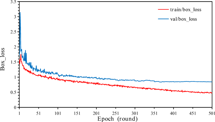
Graph of the box loss curves on the training and validation sets.
Cls loss
In object detection tasks, classification loss (cls loss) is a critical metric for evaluating the accuracy of the model’s predicted target categories. This loss function assesses the discrepancies between the predicted class labels and true class labels, thereby optimizing the model’s performance in classification tasks. In the YOLOv11 series models, (cls loss) is employed primarily to ensure that the model can accurately distinguish between target categories, such as by differentiating between flames and smoke in forest fire detection scenarios, as illustrated in Eq. 2.
$$\:cls\:loss=-\sum\:_{i=1}^{n}\left[{y}_{i}log\right({p}_{i})+(1-{y}_{i}\left)log\right(1-{p}_{i}\left)\right]$$
(2)
——where:
\(\:{y}_{i}\)
True class label (value of 0 or 1, indicating whether the target belongs to a specific category);
\(\:{p}_{i}\)
Probability predicted by the model that the target belongs to the category (ranging from 0 to 1);
n
Number of categories;
These results demonstrate that YOLOv11 attains high classification accuracy and robust generalization capabilities in object detection tasks, effectively enhancing the model’s applicability across various fire detection scenarios.
As illustrated in Fig. 9, the cls loss curves for both the training and validation sets can be analyzed in three distinct phases. Initially, during the early training phase (Epochs 0–25), the cls loss values for the training and validation sets start at 2.8058 and 1.7946, respectively. The cls loss of the training set peaks at 2.8058 during the first epoch, whereas the cls loss of the validation set reaches a higher peak of 4.6255 in the fourth epoch. This suggests that the model has not yet effectively learned discriminative features for classification, resulting in unstable performance. The greater fluctuation in the cls loss of the validation set further indicates a limited generalizability to unseen data at this stage.
In the middle training phase (Epochs 26–201), both training and validation cls loss values steadily decline, demonstrating that the model begins to effectively capture class-distinguishing features and improve classification performance. The continuous decrease in the training set’s cls loss reflects the model’s adaptation and fitting to the class patterns within the training data. Although the cls loss of the validation set exhibits some fluctuations in complex scenarios, the overall trend remains downward, signifying enhanced generalization performance.
Finally, in the late training phase (Epochs 201–501), the cls loss for both sets further decreases and stabilizes, with the training set’s cls loss decreasing to 0.3242 and the validation set’s cls loss to 0.5883. These values represent decreases of 88.44% and 67.22% from their initial values, respectively. This phase indicates that the model has achieved a well-converged state. Although the cls loss of the validation set is slightly greater than that of the training set, the minimal gap between them suggests that the model possesses strong generalizability when handling unseen data.
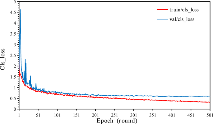
Graph of the cls loss curves on the training and validation sets.
Dfl loss
Distribution focal loss (dfl loss) is introduced in object detection tasks to increase the prediction accuracy of bounding boxes. Unlike traditional discrete coordinate predictions, dfl loss models the bounding box coordinates as probability distributions and calculates the loss on the basis of these distributions. This approach optimizes the bounding box position at the subpixel level, significantly improving the prediction precision (Eq. 3) [84]. Specifically, dfl loss predicts a continuous coordinate distribution for each bounding box boundary (such as the left, right, top, and bottom boundaries) and optimizes these distributions. This enables the model to more accurately adjust irregular and blurry boundaries of flames and smoke, thereby enhancing detection performance. The formula is as follows:
$$\:dfl\:loss=-\sum\:_{i=1}^{n}\sum\:_{j=1}^{k}[{w}_{j}. \:{y}_{ij}.\:log({p}_{ij}\left)\right]$$
(3)
——where:
\(\:n\)
Number of bounding box boundaries (e.g., left, right, top, bottom) in an image, with four bounding boxes per box.
\(\:k\)
The number of distribution intervals obtained after discretizing each boundary position;
\(\:{y}_{ij}\)
Discrete value at the j-th interval of the i-th boundary after discretizing the actual bounding box position;
\(\:{p}_{ij}\)
The probability predicted by the model for the j-th value at the i-th boundary position;
\(\:{w}_{j}\)
The weight value used to adjust the distribution accuracy.
As illustrated in Fig. 10, the dfl loss curves for the training and validation sets align with the trends observed in box loss and cls loss and can be divided into three stages:
Early training phase (epochs 0–45): The initial dfl loss values are 2.4556 (training set) and 2.7088 (validation set). The training set’s cls loss peaks at 3.1271 in the 5th epoch, whereas the validation set’s cls loss reaches 4.1895 in the 3rd epoch, indicating instability in class discrimination and weaker generalizability to unseen data.
Middle training phase (epochs 46–351): As training progresses, dfl loss decreases significantly for both datasets, reflecting improvements in learning distribution characteristics and optimizing classification and detection. The training set’s dfl loss steadily declines, whereas the validation set shows fluctuations in complex scenarios but maintains an overall downward trend, indicating enhanced generalizability. During the late training phase (epochs 351–501), dfl loss further decreases and stabilizes, reaching 1.1241 (training set) and 1.6099 (validation set), corresponding to reductions of 54.22% and 40.57% from the initial values and 64.05% and 61.57% from the peak values, respectively. The model achieves a well-converged state, with a small gap between training and validation losses, indicating strong generalizability to unseen data. This trend highlights dfl loss’s role in achieving high-precision detection, particularly in complex scenarios such as flames and smoke, enhancing YOLOv11’s applicability in diverse object detection tasks.
To further support the visual interpretation of the training curves, Table 3 provides a comprehensive numerical summary of the three core loss functions—box loss, classification loss, and distribution focal loss—on both the training and validation sets. The table presents the initial values, maximum values (with corresponding training rounds), final values, and relative drop rates. These quantitative metrics reinforce the graphical findings, demonstrating a consistent and substantial decrease across all loss components as training progresses. Notably, the classification loss on the validation set decreased by over 67%, and the box loss showed a reduction of nearly 70% on the training set, indicating effective convergence and improved generalization capability.
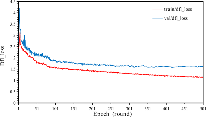
Graph of the dfl loss curves on the training and validation sets.
Evaluation and analysis of the accuracy metrics
In object detection tasks, commonly used accuracy metrics for evaluating model performance include precision, recall, mAP < sub > 50 (mean average precision at an IoU threshold of 50%), and mAP < sub > 50–95 (mean average precision across multiple IoU thresholds). These metrics assess the model’s accuracy in locating and classifying targets, coverage, and overall detection capability. Precision is defined as the proportion of true positive predictions among all positive predictions made by the model (Eq. 4). Recall measures the proportion of true positive detections out of all actual positive samples (Eq. 5). mAP < sub > 50 represents the model’s average precision at an IoU threshold of 0.50, calculated as (Eq. 6)65. mAP < sub > 50–95 is the average precision calculated across multiple IoU thresholds ranging from 0.50 to 0.95 with a step size of 0.05, as shown in Eq. (7)65.
$$\:Precision=\frac{TP}{TP+FP}$$
(4)
$$\:Recall=\frac{TP}{TP+FN}$$
(5)
$$\:{mAP}_{50}=\frac{1}{N}\sum\:_{i=1}^{N}{AP}_{50,i}$$
(6)
$$\:{mAP}_{50-95}=\frac{1}{N}\sum\:_{i=1}^{N}\frac{1}{K}\sum\:_{j=1}^{K}A{P}_{i,j}$$
(7)
——where:
TP (true positive): the number of samples correctly predicted as positive.
FP (false positive): the number of samples incorrectly predicted as positive.
FN (false negative): the number of samples incorrectly predicted as negative.
N: Total number of target categories.
AP50,i
Average precision for category i at an IoU threshold of 0.5.
K
Number of different IoU thresholds (10 values from 0.5 to 0.95).
APi, J
Average precision for category i at the j-th IoU threshold.
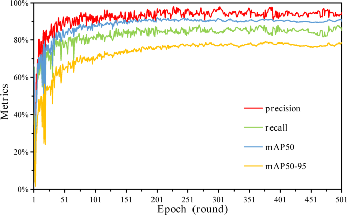
The various accuracy curves of the metrics.
Figure 11 shows the curves of different metrics on the training and validation sets. The precision initially decreases from 0.664 to 0.076 during the early training phase (epochs 0–25) and then gradually increases to 0.949, indicating a reduction in the model’s false positive rate and a significant improvement in classification accuracy. Recall decreases from an initial value of 0.619 to 0.193 and then steadily increases to 0.850, reflecting a substantial enhancement in the model’s ability to capture positive samples and a significant reduction in false negatives. mAP < sub > 50 decreases from 0.668 to 0.048 in the early training phase and then increases to 0.901, demonstrating a notable improvement in the model’s detection accuracy at a single IoU threshold. Similarly, mAP < sub > 50–95 decreases from 0.408 to 0.017, followed by an increase to 0.786, indicating a considerable improvement in the model’s comprehensive detection capability across multiple thresholds, especially under high IoU thresholds.
Overall, all four metrics initially decrease but then increase, reflecting the model’s continuous optimization of feature extraction and classification capabilities during training. This progression gradually enhances the overall detection performance and generalizability of the model. Precision and recall directly indicate the model’s fundamental classification capabilities, whereas mAP < sub > 50 and mAP < sub > 50–95 provide a more comprehensive evaluation of the model’s detection performance under varying degrees of overlap. In particular, mAP < sub > 50–95 imposes greater demands on the model’s comprehensive detection ability, underscoring its effectiveness in diverse scenarios.
Evaluation and analysis of F1 score
In the research and application of deep learning-based forest fire smoke recognition object detection technology, F1 Score is a key metric for evaluating classifier performance, particularly with imbalanced datasets (e.g., in forest fire detection, smoke occurrences are much less frequent than background images). The F1 Score is the harmonic mean of precision and recall, providing a balanced evaluation of model performance by considering both false positives and false negatives. Its formula is shown in Eq. 8.
$$\:F1\:Score=2\times\:\frac{Precision\times\:Recall}{Precision+Recall}$$
(8)
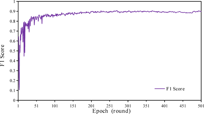
Analyzing the trend of the curve, the model’s performance fluctuated significantly in the early stages (the first 10 epochs), with a sharp drop to a minimum value of 0.1089 in the 4th epoch (Figure 12). This could be due to unstable initial model weights or performance degradation caused by an excessively high learning rate. However, after this stage, the model quickly recovered and improved, demonstrating its ability to capture key data features in a short time. After 50 epochs, the F1 Score stabilized above 0.8 and gradually became steady. By approximately 200 epochs, the F1 Score showed minimal fluctuation, indicating that the model was nearing convergence. By the end of training, the final F1 Score reached 0.8968, marking a 39.96% improvement from the initial value and a dramatic 723.72% increase from the 4th epoch’s minimum value. This highlights the model’s exceptional smoke detection ability after training. In the context of forest fire smoke recognition, an F1 Score close to 0.9 indicates high detection precision and recall, effectively minimizing the risks of false positives and false negatives, and meeting the dual requirements of high accuracy and real-time performance for practical applications. Early performance fluctuations may be due to factors such as uneven data distribution, initial weight settings, or a high learning rate. As training progressed, the model adapted to the complex features of forest environments, exhibiting strong robustness in smoke detection.
As a complement to the F1 score and accuracy trend analyses presented earlier, Table 4 summarizes the numerical progression of major evaluation metrics, including precision, recall, [email protected], [email protected]:0.95, and F1 Score. For each metric, the table lists the initial values, observed minimums during early epochs (where applicable), and the final values upon training completion. Additionally, percentage improvements from both the initial and lowest values are calculated. The F1 Score improved by nearly 40% from its initial state and over 720% from its minimum, while [email protected]:0.95 nearly doubled, reflecting a significant boost in detection robustness and consistency. These results further validate the effectiveness of the YOLOv11 model in handling complex detection tasks such as forest fire smoke recognition.
Evaluation and analysis of precision-recall curves
In this study, the precision‒recall curve (PR curve) is utilized to illustrate the trade-off between precision and recall under varying threshold conditions during the detection of flames or smoke. By adjusting the detection threshold, the values of precision and recall change, enabling the plotting of a comprehensive PR curve. Typically, the shape of the PR curve provides an intuitive assessment of the model’s performance: a curve positioned in the upper right corner and resembling a square indicates excellent performance in both precision and recall, whereas a curve situated in the lower left suggests poor model performance. By analyzing the shape of the PR curve, the model’s performance across different thresholds can be evaluated, and the optimal threshold can be selected to optimize the prediction results. Furthermore, the area under the PR curve represents the average precision (AP) for that category. [email protected] measures the overall performance of the model by averaging the AP values across multiple categories at an intersection over union (IoU) threshold of 0.5. Specifically, under the condition of IoU ≥ 0.5, [email protected] assesses the model’s comprehensive performance across different categories by calculating the mean of the areas under each category’s PR curve. A higher [email protected] value signifies stronger overall performance in detection tasks. As depicted in Fig. 13, the evaluation of the PR curve reveals that the model achieved an average [email protected] of 0.901, demonstrating high detection accuracy. Although the [email protected] values vary among different categories, the smoke category attained an [email protected] of 0.962, whereas the flame category reached 0.841. Notably, despite the slightly lower precision of the flame category than the smoke category, an [email protected] of 0.841 represents outstanding performance in flame detection. Flames present high detection difficulty because of their variable shapes, complex features, and strong dynamics. Nonetheless, the model maintains high precision in detecting such complex targets, underscoring its robustness and recognition capabilities. These results indicate that YOLOv11 exhibits excellent detection performance and has significant application potential across various fire scenarios.
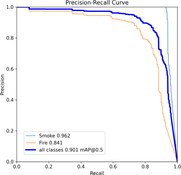
Precision‒recall curves.
Comprehensive evaluation and analysis of test set results
Confidence is a key metric for assessing detection reliability, indicating the model’s confidence in the presence of a target and its classification within the predicted bounding box. The definition of confidence, shown in Eq. 11, is determined by two primary factors: the predicted probability of the target class and the alignment between the bounding box and the target’s true position. It represents the model’s confidence in predicting a specific target, derived from the training data as a probability value, typically ranging from 0 to 1. The closer the confidence value is to 1, the more confident the model is in detecting the target; conversely, the closer the confidence value is to 0, the more the model believes there is no target in the image or that the prediction is unreliable.
$$\:Confidecne=P\left(Object\right)\times\:Clsaa\:Probability$$
(11)
——where:
P(Object)
The probability that an object exists within the predicted bounding box, indicating the model’s confidence that the detection box contains an object.
Class probability
The likelihood that the detected object belongs to a specific category, assuming the object is present.
In object segmentation tasks, confidence typically represents the model’s degree of certainty regarding a particular detection result, quantified as the probability that the model considers the detection to be correct. Higher confidence implies greater certainty in the accuracy of the detection results, which is usually associated with higher precision, indicating a lower false positive rate at high confidence levels. Conversely, lower confidence suggests less certainty in the model’s judgments, increasing the likelihood of false positives or false negatives. Therefore, confidence serves as a crucial metric not only for evaluating the model’s certainty in individual detection results but also for reflecting the model’s overall detection performance across different confidence thresholds.
As illustrated in Fig. 14, within the test set, 86.89% of the samples have confidence scores exceeding 0.85, indicating that the model is highly confident in the detection results of the majority of samples. However, performance varies across different target types (flames and smoke). The average confidence for flame detection is 0.90, whereas for smoke detection, it is 0.88, indicating that the model is more certain in detecting flames than in detecting smoke. To determine if these differences are statistically significant, a t-test was conducted on the confidence scores for flames and smoke. The results show that the difference in average confidence between flames (72.21%) and smoke (78.87%) is statistically significant (p < 0.05), indicating that the model is significantly more confident in detecting smoke than flames. This difference may stem from the distinct visual characteristics of flames and smoke: flames typically possess more defined shapes and color features, whereas smoke exhibits more uncertain and variable shapes and textures. This variability poses greater challenges for the model in accurately detecting smoke, resulting in slightly lower confidence scores. These findings suggest that although the model demonstrates high overall confidence in detections, there are subtle differences in performance across different target types. This highlights the necessity for further optimization of the model to increase the detection accuracy for complex targets such as smoke.
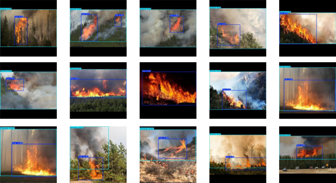
Example of the test set samples.
link

