Prediction of high-risk pregnancy based on machine learning algorithms

2.1 Research process

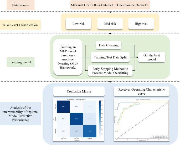
This study harnessed the open-source MHRD from Bangladeshi medical institutions, covering multiple hospitals, community clinics, and maternal healthcare centers, and encompassing data on 1014 pregnant women. Records of pregnant women aged 10–18 years were excluded due to ethical concerns and data sparsity, ensuring the dataset’s clinical validity. Risk levels are stratified into low, medium, and high categories. Post-data preprocessing, the dataset is randomly divided into a training set of 362 and a test set of 90, adhering to an 8:2 ratio. To curb overfitting in the MLP model, early stopping is employed¹³. The model’s predictive accuracy is gauged through a confusion matrix and Receiver Operating Characteristic (ROC) curve, with the research flowchart delineated in Fig. 1.

Data distribution

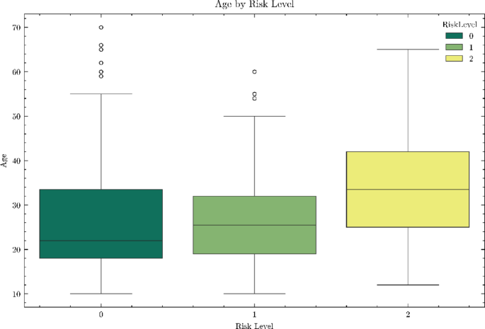
The input features include maternal age, systolic blood pressure, diastolic blood pressure, blood glucose levels, body temperature, heart rate, and risk level. These features were selected based on their established medical relevance to pregnancy risk assessment. After data cleaning and deduplication, a total of 452 data entries were obtained in this study, including 234 low-risk entries, 106 medium-risk entries, and 112 high-risk entries. The data distribution is shown in Fig. 2.

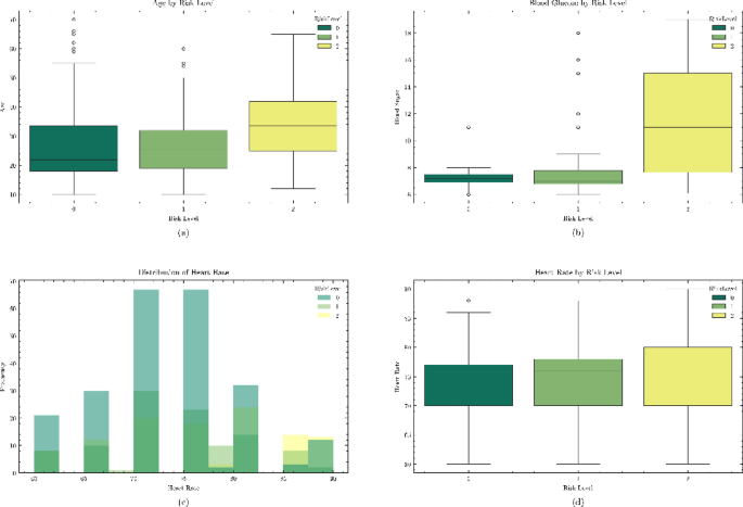
In Fig. 3, there are three box plots and one histogram. Figure 3a, b, d are box plots representing the distribution of age, blood sugar, and heart rate across different risk levels in the dataset, respectively. Figure 3c is a histogram showing the distribution of risk levels corresponding to different heart rates. From Fig. 3a–d, it is evident that individuals with a high pregnancy risk level have higher age, blood sugar, and heart rate compared to those with medium and low risk levels, which aligns with medical objective principles.

Distribution chart of risk levels for different ages, blood sugar, and heart rates.

Machine learning methods

Six machine learning algorithms—MLP, LR, DT, RF, XGBoost, and SVM—are employed to construct predictive models. It is worth noting that MLP demonstrates superior performance compared with the other five algorithms. This choice is based on the comprehensive evaluation of each algorithm’s performance in terms of accuracy, precision, and other relevant metrics. In this study, we’ve adopted a multifaceted strategy to refine the accuracy and generalization of our MLP model, which includes data preprocessing, the application of the SMOTE algorithm to address class imbalance, and the implementation of early stopping to prevent overfitting. The MLP model consists of three hidden layers, with 256, 128, and 64 neurons respectively. All hidden layers utilize the ReLU activation function and are followed by a SoftMax output layer. To prevent overfitting, Dropout layers with a dropout rate of 0.5 are inserted after the first two hidden layers. The model was trained using the Adam optimizer with a learning rate of 0.001 and a cross-entropy loss function. The batch size was set to 32, and the maximum number of training epochs was 10,000. Training would be halted if the validation loss did not improve for 300 epochs.

Our data cleaning process was essential for ensuring data quality, where we removed erroneous, duplicate, or irrelevant information from the open-source dataset from Bangladesh, including outliers such as records of pregnant women aged between 10 and 18 years. We quantified risk levels numerically, assigning values of 2, 1, and 0 to high, medium, and low risks, respectively, to facilitate subsequent analysis. To accurately assess model performance, we divided the dataset into a training set, comprising 80% of the data, and a test set, comprising 20%, using stratified random sampling to maintain the distribution of each category across both sets. To combat overfitting and enhance the model’s ability to learn from the minority class, we applied the SMOTE algorithm and introduced Dropout layers within the MLP model. We applied SMOTE exclusively to the training set post-split to avoid data leakage The test set remained unmodified to ensure unbiased evaluation. Additionally, we employed early stopping with a patience parameter P, which monitors performance on the test set and halts training if there’s no improvement for P consecutive epochs, reverting the model to its best-performing state. This approach not only prevents overfitting but also ensures that the model retains its peak performance.

For model interpretability analysis, we utilized a confusion matrix and ROC curve to assess the performance of the optimal model. The confusion matrix provides a clear view of the model’s predictive accuracy, while the ROC curve offers an intuitive representation of the model’s overall performance by comparing true positive and false positive rates across various thresholds. These methods validate the model’s risk level predictions and enhance the interpretability of the results, thereby ensuring the reliability of our predictions.

Experimental platform

This study was conducted on a computer equipped with an NVIDIA GPU RTX3050Ti, a CPU model AMD Ryzen 7 5800H, and 1.5TB of disk space. All experiments were based on the Python programming language. To build and train the MLP model, TensorFlow (2.18.0) and Keras (3.6.0) libraries were used. Data processing and analysis benefited from Pandas (2.2.3) and NumPy (1.24.4), while data visualization was performed using Matplotlib (3.5.1). Model optimization was achieved using Sklearn (1.5.2).