Predicting abnormal fetal growth using deep learning

Study design

In this retrospective, multi-center cohort study, we used a deep learning model for estimating fetal weight based on ultrasound images obtained across 17 hospitals in Denmark between 2008 and 2018. Birth weight data were obtained through the Danish Fetal Medicine Database, and imaging data were collected from four central servers. The Danish Patient Safety Authority, Islands Brygge 67, 2300-Copenhagen, Denmark, waived patient consent for this study (Record No. 3-3013-2915/1), and the Danish Data Protection Agency, Carl Jacobsens Vej 35 2500-Valby, Denmark, approved the study (Protocol No. P-2019-310).

The Hadlock formula is based on measurements of Abdominal Circumference (AC), Head Circumference (HC), and Femur Length (FL) performed by the clinician during the scan. The measurements were obtained automatically using Optical Character Recognition (OCR). For more detail refer to Supplementary Material G.

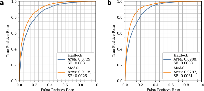
The confidence intervals and standard errors for the Receiver Operating Characteristic (ROC) curves were calculated using the Hanley method^41,42.

Dataset

Images used for fetal biometry measurements often come with embedded markings placed by clinicians during the scan. One example of such marking can be seen in Supplementary Fig. 6a, where calipers (yellow crosses) are placed on the picture to outline the anatomy to be measured, and the result is placed in a table in the lower-right corner. The table contains the value and the code of what is being measured: FL, AC, HC, and Biparietal Diameter (BPD).

These measurements were performed by the sonographers and clinicians on the three standard ultrasound planes required for estimating fetal weight and served as an input to the Hadlock formula. All 17 hospitals follow the international criteria for obtaining standard planes (ISUOG criteria for 3rd trimester ultrasound), and measurements are performed according to national guidelines (dfms.dk).

Optical Character Recognition (OCR) based on Tesseract was used to automatically classify the images as head, abdomen, femur, and other and extract the relevant measurements. The “other” class was discarded. Next, the images were aggregated based on the patient’s identification number and study date to obtain sets of images from the same examination. Furthermore, sets that did not have at least one image from each class were excluded. Lastly, fetal weight at scan time was extrapolated from the birth weight using the Marsal growth curve²⁵.

The data was limited to singleton pregnancies only and was divided on a patient basis between training, validation, and test sets (85%,5%,10%), ensuring no patient overlap. In the event that multiple images of each anatomical region (femur, abdomen, head) were obtained during an examination, multiple observations were created by generating all feasible permutations of the available images. The training included 27% of 2nd-trimester images to increase the amount of training data. However, the test set contains only 3rd-trimester images with gestational age above 28 weeks. Before training, the calipers were removed from the images to avoid shortcut learning, see Supplementary Material G.

The standard deviation of the fetal weight is not fixed and varies as a function of the weight itself. Similarly, as in Maršál et al., it was set to 12%. Therefore, the standard score is calculated \(z=\frac{x-\mu }{0.12\mu }\). Moreover, fetuses with a fetal weight below the 10th percentile (z < −1.282) are referred to as SGA, while fetal weights above 90th (z > 1.282) are referred to as LGA. Normal weight fetuses are referred to as AGA.

Model

The model used in this study was based on RegNetX 400 Mf⁴³ and was comprised of two distinct parts. The first part of the model processed the images to generate a measurement of the input anatomical structure and an embedding vector that corresponded to this structure. This vector enabled the model to encode additional information about the input images beyond the measurements. The entire model was composed of three subnetworks, each responsible for processing a different standard plane (head, abdomen, femur).

The second part of the model was composed of two fully connected layers that accepted the predicted measurements and embedding vectors. The output was the Estimated Fetal Weight (EFW). The block diagram of the model can be seen in Supplementary Material C.

Lastly, the anatomy presented on an ultrasound image can vary in scale depending on the zoom level chosen by the operator. To alleviate this problem, pixel spacing (spatial resolution) was input into the first part of the model to provide information about the relative scale of the image. This parameter is saved in the DICOM files exported from the ultrasound machine.

Training

The models were trained using the AdamW optimizer with a learning rate of 1e-4, weight decay of 1e-6, and batch size of 8. To reduce training time, the RegNetX parameters obtained from training on ImageNet data⁴⁴ were used as a starting point. The training images were center cropped and resized to 224 × 224px, converted to grayscale, and further augmented with random rotation (±25^∘), shear (±10^∘); translation (0.05 of image size); brightness (0.2), contrast (0.2), and random horizontal flip (P = 0.5). The model was trained using a multi-task learning scheme to output the measurements: HC, BPD, AC, FL, and EFW. Images as well as all measurements were normalized to fit 0 to 1 interval.

In our study, we incorporated an additional weighting parameter into the loss function used for estimating fetal weight predictions. Specifically, we utilized relative error as the base loss function and added a weighting parameter based on the z-score to further emphasize the loss on abnormal fetuses. This is illustrated in Equation (1). The same loss function was also utilized for the measurement predictions.

Where:

• y_i = fetal weight based on Maršál growth curve²⁵

• \(\widehat{{y}_{i}}\) = Estimated Fetal Weight (EFW)

• z_i = fetal weight z-score

The training dataset is organized such that each unique scan corresponds to one entry, but the scans can contain more than one image of each standard plane. Therefore, during training, a set of three images (head, abdomen, and femur) is randomly sampled from each scan.

Uncertainty estimation

Test time augmentation⁴⁵ was used to estimate prediction uncertainty. Each set of images was augmented 10 times and passed through the model to obtain multiple predictions for the fetal weight; the standard deviation of the predictions is used as the initial uncertainty estimate. The augmentation parameters used in this step were the same as the ones used in training.

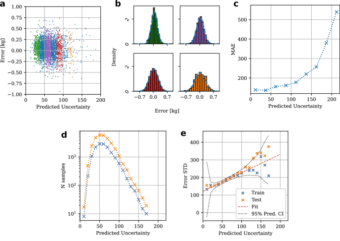
Values obtained in this way correlate with the prediction errors, as detailed in Fig. 4: Figure 4a shows the distribution of errors. Moreover, to evaluate how the prediction error changes as a function of predicted uncertainty, the data was divided into bins with a width of 10. In Fig. 4a, 4 out of the 22 bins are highlighted in color, and Fig. 4b shows the distribution of errors in those same bins. Notice that the errors in bins are normally distributed and that the standard deviation increases as the uncertainty increases. Additionally, Fig. 4c shows the mean absolute error.

a Predicted uncertainty is plotted vs. prediction error and binned into levels of predicted uncertainty, indicated by color. b For every second bin from (a), indicated by color, we show how higher predictive uncertainty comes with a broader distribution of predictive errors. c The Mean Absolute Error (MAE) grows with increased predicted uncertainty. d, e The STD of the prediction error (e) matches the smaller samples (d) found in the same predicted uncertainty bins.

Next, the error standard deviation in each bin was paired with the mean predicted uncertainty in that bin. Using the number of samples, shown in Fig. 4d, as a weighting factor, a weighted linear regression model was fitted to this data as shown in Fig. 4e. This linear relationship can be utilized to convert the uncertainty to the scale of the errors.

Analysis of pixel-level information

Saliency heatmaps were developed as described in Supplementary Material E. A subset of the test data (1800 images of the transthalamic, transabdominal, and the fetal femur) was analyzed by two feteal medicine clinicians. The two most intensely highlighted regions of each image were annotated, and the frequency of different anatomical features was calculated across the dataset. For a detailed description of the annotation protocol, please see Supplementary Material B.