Modeling saturation exponent of underground hydrocarbon reservoirs using robust machine learning methods

Modeling background

In this part, the description of each machine learning algorithm utilized in the current study is put forward.

Decision tree

Decision Trees represent a powerful suite of machine learning algorithms designed for classification and regression tasks²⁵. Developed to categorize and make predictions on previously unseen data, the Decision Tree algorithm works by building a tree-like structure that recursively splits the dataset, driven by the feature that yields the highest information gain or reduction in impurity, until a pre-defined stopping criterion is met. This process culminates in a tree with leaf nodes representing the majority class or prediction for new samples. More technical descriptions along with the pertaining equations may be found in²⁶.

AdaBoost

AdaBoost²⁷ (Adaptive Boosting) is a widely-used ensemble technique that combines multiple weak learners, referred to as base estimators, to form a more powerful and accurate regressor for prediction tasks. The AdaBoost algorithm commences by fitting a base estimator to the raw data, after which it proceeds to fit additional copies of the same estimator to the data with adjusted instance weights that depend on the current prediction errors. This iterative process ultimately yields a weighted combination of the base estimators, which together constitute the boosted regressor, resulting in improved predictive accuracy²⁸.

Random Forest

The Random Forest regressor is a robust ensemble learning methodology that leverages multiple decision trees to enhance the accuracy and generalizability of the resulting model. By combining the predictions of numerous individual trees, each trained on a random subset of the data and features, the Random Forest algorithm effectively reduces overfitting and captures the underlying patterns within the data. This powerful approach to regression tasks not only yields accurate predictions but also enables the assessment of feature importance, providing valuable insights into the factors that contribute most significantly to the observed outcomes²⁹. The Random Forest algorithm has garnered substantial popularity within the machine learning domain due to its ability to deliver strong performance without requiring extensive hyperparameter tuning. Furthermore, its capacity to handle large-scale datasets makes it an attractive choice for real-world applications where data abundance can be overwhelming for other algorithms. This combination of robustness, ease of use, and scalability contributes to the widespread adoption of Random Forests as a go-to method for various classification and regression tasks across diverse domains³⁰.

Ensemble learning

Ensemble learning techniques generate a collective decision-making process by amalgamating the powers of individual learning models to achieve improved reliability. These methodologies can be characterized into non-generative and generative approaches, depending on their prediction generation strategy. Non-generative ensemble learning techniques focus on producing new predictions by integrating the outputs of independently trained models, without intervening in their learning stages. Conversely, generative ensemble learning techniques have the capability to construct the underlying learners, while also optimizing learning algorithms and datasets within the ensemble. Among non-generative ensemble learning methods, the voting ensemble and stacking ensemble techniques are the most prominent. The voting ensemble regression method calculates a final prediction by averaging the predictive outcomes of combined independent learning algorithms, thus leveraging the strengths of multiple models for enhanced predictive performance³¹.

Support vector machine

The kernel function within the support vector machine (SVM) is responsible for mapping sample data into high-dimensional space enabling the solution of nonlinear regression problems³². To ensure SVM predictive model is associated with generalization capability and prediction accuracy, parameter optimization selection, kernel function and sample data processing are the key components that needs to be delicately taken into account. In this regard, the mapping relationship between the output variable and input variables is expressed as:

In which y is the output variable and x being the input variable and n represents the number of input variables. Kernel function determines the predictive performance of SVM model. The most commonly used kernel function is called radial basis function (RBF), the details of which can be found in³³.

Multilayer perceptron artificial neural network

Artificial Neural Networks (ANNs) are powerful mathematical tools that draw inspiration from the structure and function of the human nervous system. As noted previously, the foundation of ANNs lies in mimicking the human brain’s parallel processing capabilities for uncovering intricate nonlinear relationships between independent and dependent variables. By employing interconnected layers of artificial neurons, ANNs can learn from data, adapt to new inputs, and generate accurate predictions in complex problem domains³⁴. ANNs represent sophisticated statistical tools that emulate the human nervous system’s interconnected neurons within a computational network. ANNs encompass various types and architectures, each tailored to specific tasks and problem domains. These models excel at pattern recognition and decision-making, with applications spanning numerous scientific fields. The extensive adoption of ANNs across diverse disciplines highlights their versatility and efficacy in addressing complex challenges, positioning them as a prominent tool in contemporary scientific research^35,36. The remarkable precision of ANNs positions them as highly effective nonlinear analysis tools, capable of replacing time-consuming and costly experimental procedures. ANNs have demonstrated their ability to address intricate modeling tasks, including prediction, pattern recognition, and classification, establishing their prominence in scientific research³⁷.

Methodology

Gathered data statistics

The dataset employed in this research comprises field data with 1041 datapoints of routine and special core analysis (RCAL and SCAL) as functions of absolute permeability, porosity, true resistivity, water saturation and resistivity index. The statistical properties of these data are outlined in Table 1. It is well-established within the field of petrophysics which involves geological formation properties, the rock saturation exponent is linked to above-mentioned specifications, albeit with varying degrees of correlation and directionality. Given these relationships, the input parameters used for the data-driven model development encompass absolute permeability, porosity, true resistivity, water saturation, and resistivity index as the required input factors. The output label is the saturation exponent.

Sensitivity analysis

In this part, we seek to find out the relative effect of each input variable including absolute permeability, porosity, true resistivity, water saturation and resistivity index on the output factor which is saturation exponent. This is carried out here with the consideration of relevancy factor in which it is calculated for each separate input variable. The equation of relevancy factor is defined as³⁸:

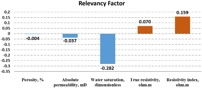
In which j denotes the specific input variable. Note that the probable range of relevancy factor lies within -1 and + 1. Also, the higher the magnitude of the calculated relevancy factor, the stronger the relationship of the specific input variable with the output variable. In addition, a negative and positive relevancy index indicate indirect and direct relationship of the so-called input variable with pertinent output variable. In this way, the estimated relevancy factor for all the considered input factors is given in Fig. 2. As can be seen, resistivity index and true resistivity are directly correlated with saturation exponent while porosity, absolute permeability and water saturation is inversely related with saturation exponent. Additionally, water saturation has the strongest relationship with output variable.

Exploring the relative impact of each variable on the saturation exponent using relevancy factor.

Outlier detection

The reliability of any data-driven intelligent model is significantly influenced by the quality of the dataset employed during the development process. To ensure the credibility of the data in this study, we apply the widely recognized Leverage technique, which involves the utilization of the Hat matrix. This matrix is defined as follows³⁸:

In the aforementioned equation, the design matrix X is denoted as an m*n matrix, where n signifies the number of input variables and m represents the total number of data points. To identify potential outliers using the Leverage technique, we employ the Williams’ plot, which visualizes the relationship between the Hat values and their normalized counterparts. Within this graphical representation, the warning leverage is determined through the following calculation³⁸:

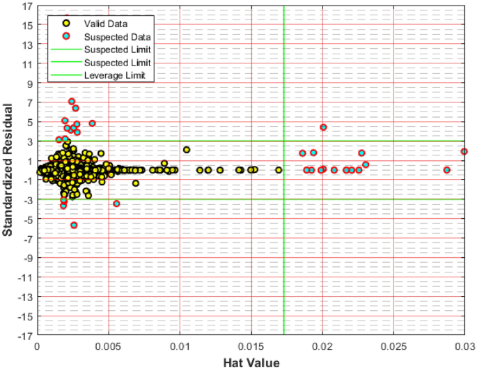
It is important to note that standardized residuals typically fall within the range of -3 to + 3. The Williams’ plot, presented in Fig. 3, facilitates the identification of outlier and suspect data points. The plot features two horizontal lines representing standardized residual values, and a vertical line indicating the warning leverage value. Data points located within these boundaries are deemed reliable and validated. As illustrated in Fig. 3, only 26 out of 1401 datapoints are classified as outliers. Despite this, all datapoints are taken into account during model development to ensure the construction of generalized models.

Identification of suspected data before intelligent data-driven modeling via Leverage methodology.

Model evaluation indices

In order to comprehend the robustness, reliability and accuracy of the developed models, the following statistical indices are estimated for each model^39,40,41:

Wherein exp and pre are known as field and estimated values, i denotes index number and the number of datapoints are depicted via N.

The input variables for the data-driven modeling include absolute permeability, porosity, true resistivity, water saturation and resistivity index for the modeling process of saturation exponent. Moreover, 80%, 10% and 10% of all datapoints are randomly selected for training, validation and testing phases, respectively. As widely known, the validation is used to avoid overfitting while testing is implemented using the unseen data during the model training (development) phase. To minimize the impact of data fluctuations during the modeling process, both input and output variables are normalized using the following relationship:

Where the real value is denoted by n, subscripts max and min signify maximum and minimum value of the dataset and subscript norm is known as the normalized value.