
Identifying diseases symptoms and general rules using supervised and unsupervised machine learning

In this section, we analyze data to investigate disease symptoms using AR and predictive modeling.
Data preparation
As shown in Table 1, blood pressure and cholesterol level characteristics are nominal data type. Hence, we use the transformation method and encoding to have Binary variables that are then treated as numeric. On the other hand, in JMP software, to perform AR mining, the data needs to be in list format, and then it should be transformed to nominal format type. In this respect, we treated each patient as a single transaction. Then, we divided the dataset into three groups based on the patient’s age to transform a list format including: young adult, middle-age adults, and older adults. We initially applied AR mining to symptom data and identified symptom rules. Additionally, to identify and mange outliers, we apply the KNN (K = 8), robust principal component analysis (with lambda = 0.107 and outlier threshold = 2), T2, Mahalanobis, and Jackknife distances methods. Generally, results show that the rows of 1, 81, 122, 213 are outlier and should be excluded. Note that KNN identifies outliers based on distance to each observation nearest neighbors for theses rows as well as 39 rows that we ignore it. Figure 2 shows outliers using T2, Mahalanobis, and Jackknife distances for instance.

Outlier plot for the T2, Mahalanobis, and Jackknife distances methods.
After data preparation phase, we perform a descriptive statistical analysis to help more ML methods. Some of these investigations are provided here. In this regard, the dataset does not exhibit significant skewness, with only a few outliers present, and the gender distribution in the dataset is relatively balanced. Figure 3 shows that individuals have a higher likelihood of testing positive for diseases, in older age. Additionally, Fig. 4 shows fever is a main symptom of these diseases. This figure demonstrates many individuals, regardless of the type of experience (positive or negative), report coughing.
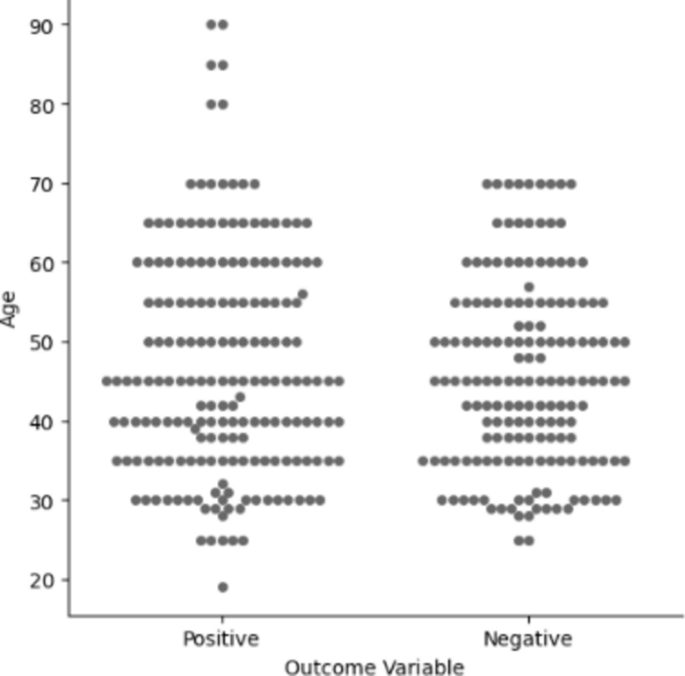
Plot of outcome results in terms of age factor.

Bar graph of some symptoms of the diseases.
The more analytics using pie chart shows the majority of the individuals in the study have high blood pressure and cholesterol. Additionally, out of 348 patients, 185 tested positive for a disease. Only 23 of the positive cases developed all symptoms. The average age of the patients is 46, with the majority being middle-aged. However, positive cases are proportionally higher in older adults. A violin plot indicates that older adults have high blood pressure, but older adult to middle-aged patients also exhibit high blood pressure. The most common symptoms were fatigue (139 cases), fever (109 cases), breathing difficulty, and cough (both seen in 88 cases). Females are more prone to the diseases than Males.
AR in unsupervised ML
We used an a Apriori method to extract lift matrix-based strong rules. Symptom transactions are part of the AR mining which aims to identify frequent item sets that meet a minimum threshold. To achieve this, we set the minimum confidence level to 1, ensuring that all generated rules have a 100% confidence level. Additionally, we establish a minimum support threshold above 0.01 and a lift greater than 4 for positively correlated rules. This means that the rules generated must have a support value greater than 1% and a lift value greater than 4, indicating a strong positive correlation between the antecedent and consequent items. Furthermore, we limit the maximum number of antecedents to 3 and the maximum rule size to 4, ensuring that the generated rules are concise and interpretable. To do so, we discover many significant AR for the data, and the top 20 symptom rules by highest lift values are given in Table 2. Table 2 concentrates on the antecedents (diseases) associated with the consequents (symptoms) to predict asymptotes of diseases.
Table 2 shows diseases strongly linked to symptoms with a confidence of 100% (except for rule 18) and a lift greater than 1. A confidence level of 100% indicates a high degree of certainty. Lift measures the performance of an AR as a response enhancer. Lift values greater than 1 indicate interdependence between conditions and their outcomes, emphasizing positive relationships. Based on rule 2, if a patient had Chronic Obstructive Pulmonary Disease (COPD) (condition), then this patient had a higher confidence for breathing difficulty in older adults’ group (consequent). Specifically, Rule 1 suggests a positive association between Typhoid fever, high cholesterol, and fatigue, while rule 10 indicates that Hepatitis B increases the likelihood of coughing, fatigue, and high cholesterol. The results also demonstrate that demographic factors impact the relationships between symptom patterns and disease types. Additionally, the proposed model seeks to predict the potential disease of a patient based on their specific symptoms. In this regard, the 20 top rules are given in Table 3.
The associations in Table 2 exhibit a high confidence and a lift greater than 1, indicating a positive links. For example, Table 3 shows 5 rules related to COPD with a 100% confidence level and a notably high lift. According to these rules, older adults experiencing breathing difficulty, fever, high blood pressure, high cholesterol, and fatigue have a 67% chance of having COPD. Similarly, the presence of high cholesterol, high blood pressure, and breathing difficulty in older adults may indicate a higher likelihood of Rheumatoid Arthritis. Additionally, the model aims to predict potential diseases based on specific symptoms, while also considering the influence of demographic factors on symptom-disease associations. Furthermore, the unsupervised algorithm can identify relationships between symptoms and various attributes, aiding in the discovery of symptom relationships. In this respect, 25 rules are extracted in Table 4.
According to Table 4, among all rules, fever was the most common consequent. To describe the extracted rules, we focus on one rule for instance. Based on rule 1, if a patient has breathing and coughing problems and high blood pressure there is a 100% confidence that he or she had a fever. Similarly, Rule 2 highlights that when a patient experience both fatigue and high cholesterol, they will also have a fever. Moreover, the last rule shows that male patient with breathing difficulty who are strongly associated with fever, with a confidence of 90%. In general, our analysis from Tables 2–4 shows that the older adults age group strongly correlated with diseases occurrence. Another analytic can be achieved from AR mining, gives in Table 5 in which the disease may be occurred in specified age are shown. To sum up, we provide some of the ages in this respect.
Moreover, we can identify diseases that have an affinity for each other using Singular Value Decomposition (SVD). Diseases that exhibit overlap, based on the SVD method, can be identified by leveraging the SVD technique. This approach decreases the dimensionality of the data, allowing for the grouping of similar diseases and the extraction of relevant information. Figure 5 and Table 6 show points or diseases that are close to each other.

Item SVD plots for the data set.
Predictive modeling in supervised ML
Now, we aim to develop a model that can accurately predict diseases using the disease symptoms and patient profile dataset. As aforementioned, this dataset contains valuable information on symptoms, demographics, and health indicators, which can be used to reveal fascinating connections and patterns. After examining the “Disease” column, we found that many unique diseases have only 1 to 5 samples, which is insufficient for a reliable disease prediction model. Predicting diseases with such limited information could lead to inaccurate results and misdiagnosis, which we want to avoid. Therefore, we will focus only on the diseases that have 10 or more samples to ensure the robustness of our model. This decision will reduce the number of cholesterol asses we are predicting down to 6, making our model more accurate. On the other hand, using checking for and handling missing values and identifying and removing duplicate entries we can ensure that our data is accurate, complete, and ready for further analysis or model building. After cleaning our data, we have focused on diseases with 10 or more samples. Understanding the balance of cholesterol asses is crucial as it can impact the performance of our ML model. To visualize this, we have utilized a pie chart in Figure 6. This step is essential for ensuring that our model is trained on a well-balanced dataset, which can ultimately enhance its predictive accuracy and reliability.

Pie chart for initial diseases classification.
The pie chart shows that the classes are imbalanced, and we need to handle class imbalance. Before that, we need to process our categorical variables to perform a univariate analysis. This analysis will help us understand the distribution of our variables and their individual impact on disease prediction. We will start with the age variable, followed by other variables like symptoms, gender, blood pressure, and cholesterol level.
The univariate analysis of the age variable in Fig. 7 reveals that age is a valuable feature for predicting certain diseases. For instance, if the age is greater than 80, the disease is likely to be a stroke. However, the dataset has limited samples, especially for ages greater than 80, which could make predicting new values in this age range challenging. The analysis also shows that some diseases like Migraine and Hypertension are not present in ages between 20 and 30, suggesting that these conditions are more prevalent in older age groups. Hypertension and Osteoporosis appear more frequently as the age increases, indicating a potential correlation between these diseases and age. Also, cholesterol levels and blood pressure, significantly influence disease prediction. For example, High blood pressure is associated with the absence of stroke, which is crucial for stroke prediction. These observations emphasize the importance of these variables in predicting diseases. The next step is to examine how these variables correlate with each other, which can help identify patterns and potential multicollinearity, ultimately influencing the model’s performance.

Bar graph of age-diseases.
Figure 8 shows that none of the variables have a strong correlation with the “Disease” variable. The most correlated variables are “Age” and “Difficulty Breathing”, with scores of 1 and − 1, respectively. In situations where there are multiple variables with high correlation scores, ML can be a viable alternative for prediction tasks. However, it’s essential to consider that ML algorithms, typically require large amounts of data to perform optimally. In our case, we have only 79 data points, which is relatively small.

Correlation of each feature in the dataset using the heat map generated by JMP Pro 17 (version 17.2.1, available at https://www.jmp.com/).
For hyperparameter tuning, we used the Grid Search method in JMP. Grid search is a simple and effective method for finding the optimal combination of hyperparameters by systematically varying each hyperparameter over a range of values and evaluating the performance of the model at each combination. We used a grid search with 10 iterations to find the optimal combination of hyperparameters for each model. For example, for the SR, we used a grid search to optimize the following hyperparameters:
-
Stepwise selection: We used a grid search to optimize the stepwise selection method. We varied the number of features to include in the model from 1 to 10, and evaluated the performance of the model at each combination.
-
Lambda: We used a grid search to optimize the lambda value, which is a hyperparameter that controls the strength of the regularization term in the model. We varied the lambda value from 0.1 to 1.0, and evaluated the performance of the model at each combination.
For the SVMs, we used a grid search to optimize the following hyperparameters:
-
Kernel: We used a grid search to optimize the kernel function, which is a hyperparameter that controls the shape of the decision boundary in the model. We varied the kernel function between linear, polynomial, and radial basis functions, and evaluated the performance of the model at each combination.
-
Gamma: We used a grid search to optimize the gamma value, which controls the width of the kernel function. We varied the gamma value under (0.1–1) and evaluated the performance of the model at each combination.
For the BF model, we used a grid search to optimize the following hyperparameters:
-
Number of trees: We used a grid search to optimize the number of trees in the forest that controls the complexity of the model. We varied the them under (10–100), and assessed the performance of the model at each combination.
-
Max depth: We used a grid search to optimize the maximum depth of the trees, which is a hyperparameter that controls the complexity of the model. We varied the maximum depth from 5 to 10, and evaluated the performance of the model at each combination.
For the BT model, we used a grid search to optimize the following hyperparameters:
-
Number of iterations: We used a grid search to optimize the number of iterations in the boosting algorithm, which is a hyperparameter that controls the complexity of the model. We varied the number of iterations from 10 to 100, and evaluated the performance of the model at each combination.
-
Learning rate: We used a grid search to optimize the learning rate that controls the step size in the boosting algorithm. We varied it under (0.1–1) and evaluated the performance of the model at each combination.
For the NB methods, we used a grid search to optimize the following hyperparameters:
-
Number of hidden layers: We used a grid search to optimize the number of hidden layers in the neural network, which is a hyperparameter that controls the complexity of the model. We varied the number of hidden layers from 1 to 3, and evaluated the performance of the model at each combination.
-
Number of neurons: We used a grid search to optimize the number of neurons in each hidden layer, which is a hyperparameter that controls the complexity of the model. We varied the number of neurons from 10 to 100, and evaluated the performance of the model at each combination.
To conduct a fair comparison between different classifiers and identify the superior model with the best performance, we have considered and calculated several evaluation metrics that are well-suited for our specific case and dataset. The evaluation metrics we have included are:
$$ \textAccuracy = \frac\left( TP + TN \right)\left( TP + TN + FP + FN \right), $$
(4)
$$ \textPrecision = \fracTP\left( TP + FP \right), $$
(5)
$$ \textRecall = \fracTP\left( TP + FN \right), $$
(6)
$$ \textF1 – \textscore = \frac2.TP\left( 2.TP + FP + FN \right), $$
(7)
$$ \textMCC = \frac{2^\left( TP.TN – FP.FN \right) }\sqrt \left( TP + FP \right).\left( TP + FP \right).\left( TN + FP \right).\left( TN + FN \right) . $$
(8)
This is a crucial measure for evaluating imbalanced multi-class classification problems. A comparative assessment of most common used ML classifiers is performed in Table 7 for analyzing and classifying diseases.
We used the confusion matrix to calculate different metrics, and the best results are marked in bold. As illustrated by Table 7, SR method is the superior model leading to the best performance with the accuracy of 86.73% (95% CI 82.69–90.71) and the precision of 75.36%. Besides, the corresponding criteria of recall and F1- measure and (Matthews Correlation Coefficient) MCC are 77.87, 81.31, and 54.02%, respectively. Based on these metrics, the “SR” model consistently performs well across evaluation criteria. To avoid additional complexity and keep this table simple to read, we preferred to exclude the standard deviation of each result metrics.
Overall, researchers focused on specific diseases or conditions mentioned in the dataset can utilize it to explore relationships between symptoms, age, gender, and other variables. Also, healthcare technology companies can use the proposed method based on ML methods for developing healthcare diagnostic tools. It is worth mentioning that the model shows strong performance in predicting asthma cases but struggles to predict other conditions, suggesting its potential use in a one-vs-all approach for asthma diagnosis. Notably, the training data is imbalanced, with asthma being the most frequent class. To address this, data augmentation techniques such as rotation, scaling, or adding noise could be implemented to improve the model’s accuracy in predicting less frequent diseases.
The study aims to identify common patterns and general rules across various diseases using ML techniques. By analyzing a diverse dataset, the research uncovers connections between symptoms, demographics, and health indicators, providing valuable insights for developing predictive models and early warning systems applicable to multiple diseases. It is worth noting that the decision to generalize the study across various diseases is grounded in several key considerations, including identifying common patterns, improving early detection, enhancing understanding, and practical implications. While the generalized approach offers several advantages, it is important to acknowledge that the study may not capture disease-specific nuances or rare symptoms that are unique to particular diseases. Future research could focus on validating the identified patterns and rules in specific disease contexts or exploring the applicability of the findings to rare or understudied diseases. In conclusion, the decision to generalize the study across various diseases is justified by the potential benefits of identifying common patterns, improving early detection, enhancing understanding, and providing practical implications for healthcare professionals. However, the limitations of this approach should be considered, and further research is needed to validate and refine the findings in specific disease contexts.
To improve the model’s ability to adapt to new, emerging diseases or changes in symptom presentation, the following strategies can be implemented in our approach:
We can easily implement a system to continuously collect and integrate new patient data into the training dataset, including information on emerging diseases and changing symptom patterns. The models can then be retrained on a regular cadence (e.g., monthly, quarterly) to ensure they remain up-to-date and can adapt to evolving disease landscapes. Additionally, we can monitor model performance on a holdout test set to identify when retraining is necessary due to degradation in predictive accuracy. This will help ensure the models can adapt to new, emerging diseases and changing symptom presentations. As a future research direction, we recommend exploring the use of ensemble learning techniques. Specifically, we suggest investigating the application of various ensemble methods to further enhance the ability of the proposed models.
Statistical significance
Now, we use a statistical test to compare the proposed ML to ensure the statistical significance of the results and provide a robust comparison. Overall, the non-parametric tests are safer than parametric tests since they do not assume normal distributions or homogeneity of variance. In the case where multiple algorithms are to be compared, Friedman’s test is the most interesting non-parametric statistical test. In Friedman test, the blocks of data, are considered independent. The underlying variables in the data are typically numeric in nature. The goal of this test is to determine whether there are significant differences among the algorithms considered over given sets of data. Training/Test set is generated as random sample from the population. The Friedman rank test can determine if there are significant differences in variation, central tendency, or shape among at least one pair of the populations being compared. The test determines the ranks of the algorithms for each individual data set, i.e., the best performing algorithm receives the rank of 1, the second-best rank 2, etc.; in the case of ties average ranks are assigned. The Friedman test is performed in respect of average ranks, which use \(\chi_F^2\). Consider \(r_i^j\) be the rank of the jth of k ML algorithms on ith of n data sets. The Friedman test compares the average ranks of algorithms, \(R_j^ .\) The null hypothesis states that all algorithms perform equivalently. Under this hypothesis the Friedman statistics is as follows:
$$ \chi_F^2 = \frac12nk(k + 1)\left( \sum\nolimits_j R_j^2 + \frack(k + 1)^2 4 \right), $$
in which \(\chi_F^2\) is distributed with k-1 degrees of freedom, when n and k are large enough. We can understand with comparing the corresponding statistics and \(\chi_F^2 (4)\) with α = 0.05, the null hypothesis is rejected. In this regard, average rankings of the ML algorithms over the data sets by the Friedman test are shown in Table 8.
Feature importance and scoring
In the literature, two primary strategies for feature selection are Forward Selection (FS) and Backward Elimination (BE) for our classifier. FS starts by selecting the best single feature and then iteratively adds the feature that improves performance the most. Conversely, the BE begins with all considered features and repeatedly removes the feature that reduces performance the most. We conducted a series of experiments using fivefold cross-validation. The dataset was divided into 80% training cases and 20% test cases. In each fold, the training data was used to calculate the accuracy of a random forest classifier using different sets of features. The set of features that yielded the best accuracy was retained. The results are presented in Table 9.
The features were ranked incrementally based on their importance, with the most important feature labeled as one, the next most important feature labeled as two, and so on. Features with the “ignored” tag were removed from the dataset.
In the Forward Selection (FS) and Backward Elimination (BE) methods, we observe that the “age” and “breathing difficulty” features are consistently ranked as the most important, indicating its significant contribution to the model. Furthermore, we note that the “fatigue” feature is ranked last in both FS and BE, suggesting its relatively low relevance. Additionally, the “Blood pressure” feature is either ignored or ranked last in both methods, implying its minimal impact on the model. This further validates the effectiveness of our algorithm in ranking features.
Deployment challenges
Successful deployment of the ML models developed in this study necessitates careful consideration of the challenges to ensure effective implementation and adoption in real-world healthcare settings. The integration of these models into existing healthcare systems can pose significant challenges. Healthcare organizations often have complex and diverse IT infrastructures, with various systems and platforms in place. Seamless integration of the ML models into these existing systems is crucial for ensuring efficient data flow, accurate predictions, and effective decision support. Key considerations for integration include data compatibility, security and privacy, and scalability. Additionally, effective clinician training and adoption are crucial. Clinicians may be hesitant to rely on automated decision support systems, especially if they lack understanding of how the models work or have concerns about their accuracy and reliability. To address these challenges, the following strategies can be employed:
-
• Comprehensive training: Providing comprehensive training to clinicians on the use and interpretation of the ML models, including their strengths, limitations, and appropriate applications.
-
• Transparency: Ensuring that the ML models are as transparent and explainable as possible, allowing clinicians to understand the reasoning behind the predictions and build trust in the system.
-
• Continuous feedback and improvement: Establishing mechanisms for clinicians to provide feedback on the performance and usability of the ML models, enabling continuous improvement and adaptation to user needs.
-
• Incentives and support: Providing incentives and support for clinicians to adopt and integrate the ML models into their daily workflows, such as through performance metrics or dedicated support staff.
Successful deployment of ML models in healthcare requires careful consideration of integration challenges with existing systems and effective clinician training and adoption strategies. By addressing these challenges, healthcare organizations can effectively leverage the power of ML to improve patient outcomes and enhance clinical decision-making.
link


