Federated learning with integrated attention multiscale model for brain tumor segmentation

This section offers a comprehensive summary of the proposed research and also outlines the procedures for data preparation, preprocessing, and the architecture of the UNet model that uses FL. The Fig. 2 illustrates the proposed methodology where the data is preprocessed and given to the U-Net model using FL for segmentation.

The roadmap given in Fig. 2 describes the detailed, step-by-step procedure for developing, training, and deploying an advanced brain image segmentation model with a high level of privacy protection and optimization through reinforcement-based FL. The preprocessing of the images is done and given to the Double Attention-based Multiscale Dense-U-Net along with RL-FedAvg algorithm. Such an approach may impact clinical workflows in a crucial way by being accurate and available in real-time for brain tumor diagnosis and treatment planning. Differential Privacy is used to ensure that local data cannot be reverse engineered from updated aggregated models. Gradient Clipping limits the L2 norm of the gradients such that very large updates wouldn’t occur, which might leak local data information. Update aggregation is done on the server without exposing individual model updates from devices that participated. Evaluation Metrics like Dice Coefficient is applied to measure accuracy of segmentation. Also, a higher PSNR indicates less inversed.

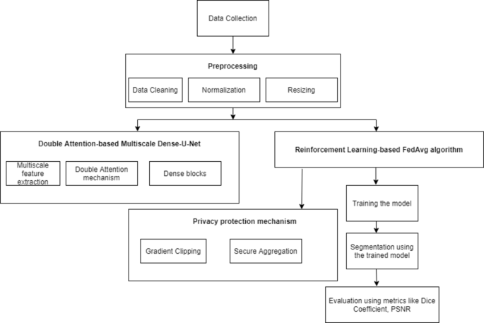
Roadmap of the proposed technique.

Preprocessing

In this work, the Keras sequence DataGenerator class is overridden to match the requirements. The `DataGenerator` class orchestrates the loading, resizing, and normalization of brain MRI images. Each MRI image, consisting of multiple modalities like Fluid-Attenuated Inversion Recovery (FLAIR) and T1-Contrast-Enhanced (T1-CE), is loaded from the specified file paths using Neuroimaging Informatics Technology Initiative (NIfTI) file format utilities. The images are then resized to a uniform dimension using OpenCV, ensuring consistency across the dataset. Normalization is applied to standardize the intensity values of the images, a crucial step for enhancing model convergence during training. By encapsulating these preprocessing steps within the `DataGenerator`, the class streamlines data preparation, ensuring that input data is appropriately formatted and optimized for subsequent training, validation, and testing stages. This streamlined preprocessing workflow enhances the model’s ability to learn meaningful features from the data, ultimately leading to improved segmentation performance.

Federated learning

In traditional machine learning or middle learning, all participating organizations (collaborators) share their training data with a centralized server. In contrast, in FL, participants train a locally shared model and communicate only updates to a central server, rather than sharing their data. The server collects and combines any changes to create a global model, after which it sends updated shared parameters to each client for further training. The FL technique enables a learning approach that trains algorithms in unity without sharing the underlying datasets, aiming to solve data governance and privacy issues. This eliminates the need for data storage and delivery in one location. Multiple collaborators in different areas can generate identical, reliable ML models. As a result, important issues such as data protection, privacy, copyright, and the use of heterogeneous data are discussed.

Centralized Learning vs. Federated Learning.

Figure 3 illustrates the Centralized Learning and FL. In Centralized Learning the data is stored in one location, making it easier to preprocess and ensure consistency. In FL the devices often have non-identical, unevenly distributed, and even biased data (referred to as non-iid data). Handling such heterogeneity can be challenging and may affect model performance. The ability of FL to protect patient privacy has attracted considerable attention in the healthcare industry. Some trust is still needed in the central server responsible for client training^31,32. A few extra elements are added to the conventional centralized training process by federated learning like:

1. 1)

   collaborator

A FL algorithm has multiple users collaborating simultaneously to train the global model. Each entity is known as a client and is just a part of the consortium that has access to any of the client’s local data.

1. 2)

   parameter server

In a FL system, the parameter/central server controls the training process. It distributes copies of the global model to its colleagues. Parameter servers and aggregators are typically associated with a single computing node.

1. 3)

   aggregator

The aggregator collects customized local images from contributors and combines them into a new global model. Federated averaging, also known as weighted averaging, is often used to combine locally generated models.

1. 4)

   round

A federation round is an interval of training stages that involves aggregating. Collaborators can train the model locally for several epochs, including incomplete epochs, within a single training round. The typical procedure for training a FL system consists of the following stages:

1. (i)

   The collaborator receives global model updates from the server, trains on personal data, and then sends local model changes to the global server.

2. (ii)

   After receiving the updated weights of the local model, the central server securely aggregates the data without gaining knowledge about any collaborators, producing a global model.

3. (iii)

   The collaborators update it locally after receiving the revised shared weights from the central server for further training.

4. (iv)

   Go back to i) for another federated round.

Overall architecture with global U-Net model.

Figure 4 demonstrates the architecture of the proposed technique with conventional U-Net. In FL, it is considered that the dataset is spread across clients \(\:m=1,\:2,\ldots M\). The notation is as follows.

There is a set of indices (Pm) of data points that signify each division for each client. Here, \(\:n\) is the total number of data points gotten by all clients, and \(\:nm\) designates the number of data points that the client currently owns, and nm = |Pm|. In this federated scenario, in mini-batch stochastic gradient descent, the calculation work for a single complete update is identified by three factors. The formula used for minimizing a loss function is indicated below:

Then, each client receives a step of gradient descent and informs its settings appropriately, dignified as:

The average loss for a stated client is computed as:

Now, let \(\:{\theta\:}_{t}^{i}\) represent the model parameters of client \(\:i\) at iteration \(\:t\), and \(\:{N}_{i}\) be the number of samples available at client \(\:i\). Then, the local update performed by a client \(\:i\) can be represented as:

Where η is the learning rate and \(\:{f}_{i}\)(\(\:{\theta\:}_{t}^{i}\)) is the local loss function at client \(\:i\) with model parameters \(\:{\theta\:}_{t}^{i}\).

The server uses average to aggregate the model updates, once each client completes their local update:

Where \(\:N\) is the total number of clients. In the proposed mixed-Fed-U-Net,

• Local models are trained independently on their respective datasets.

• The global model is constructed using FedAvg, which takes a weighted average of the weight of local models.

• The global model is updated and distributed to all participants for the next training round.

Mathematical model of federated learning with RL optimization (RL-FedAvg)

The Reinforcement Learning (RL)^4,33 is incorporated in Federated averaging model as follows:

Step 1: The global model is initialized as follows:

Then the initial global model is distributed among all clients.

Step 2: Client-side training is done with RL-optimized hyperparameters. During every round \(\:t\), the central server:

1. 1.

   Detects the present state \(\:{s}_{t}\:\)based on the performance of the client and global model metrics.

2. 2.

   Chooses actions \(\:{a}_{t}^{i}=\{{\eta\:}_{t}^{i},{B}_{t}^{i},{E}_{t}^{i}\}\) using the RL policy \(\:{\uppi\:}\left({s}_{t}\right)\).

3. 3.

   Client gets the transmitted optimized hyperparameters from the server

A local training is done by the client as follows:

Step 3: The reward is computed and the policy is updated. After training, the server assesses the client models depending upon a segmentation metric \(\:\text{M}\) and calculates the reward for every client \(\:{r}_{t}^{i}\)​. The server apprises the RL policy \(\:{\uppi\:}\left({s}_{t}\right)\) depending on the reward signal by means of a policy optimization algorithm.

Step 4: Global model is aggregated. The server collections the client models using FedAvg:

Step 5: Till convergence the process is repeated. The process is repetitive until the global model attains the wanted segmentation accuracy or until a static number of rounds \(\:T\) is finished. For image segmentation, the subsequent metrics can be utilized in the reward function \(\:{r}_{t}^{i}\)​:

where \(\:P\) is the projected segmentation mask and \(\:G\) is the computed ground truth mask.

By merging FedAvg with RL-based client optimization, this model guarantees dynamic tuning of client hyperparameters based on real-time feedback, thereby optimizing the global model for image segmentation tasks while proficiently handling client resources. The RL-FedAvg algorithm is given as follows:

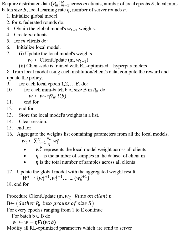
RL-FedAvg in the proposed work.

Architecture of the proposed double attention-based multiscale Dense-U-Net

The Double Attention-based Multiscale Dense-U-Net is an enhanced model of U-Net. When this proposed model is used instead of the global U-Net, it enhances the performance.

Conventional U-Net

Convolutional neural networks such as the U-net architecture are frequently used for image segmentation applications. Figure 4 represents the U-net architecture. It has been especially beneficial in the area of image analysis for medical purposes. The encoder-decoder structure of the model uses skip combinations to preserve spatial information while obtaining both local and global data. High-level features are extracted by the encoder section by successively down sampling the input image using convolutional and max-pooling layers. Two convolutional (Conv2D) layers with 32 filters and Rectified Linear Unit (ReLU) activation precede MaxPooling2D layers (\(\:2\times2\) pool size) in the encoder block, which are used for downsampling. Convolutional blocks 64, 128, 256, and 512 are convolutional blocks made up of two Conv2D layers activated by ReLU. The function of activation for ReLU can be expressed mathematically as:

As a result, for each given input \(\:x\), the output \(\:f\left(x\right)\) of the ReLU function equals \(\:x\) if \(\:x\) is non-negative and zero if \(\:x\) is negative. The U-Net architecture can be represented as in Fig. 4.

1. 1)

   downsampling layers

The number of channels can be augmented while the spatial dimensions of the feature maps are reduced with the incorporation of downsampling layers. Five downsampling layers, two input and one convolutional layer are used in this work. The forward pass of a downsampling layer utilizing convolutional algorithms and pooling is represented mathematically as follows:

The forward pass of the \(\:k\)-th layer in a neural network design is specified by this equation, particularly with regard to downsampling. It requires convolving the input feature map \(\:{h}_{k-1}\) with the weights \(\:{W}_{k\:}\) of the k-th convolutional layer, adding biases \(\:{b}_{k}\), and applying an activation function \(\:f.\) The resulting output feature map \(\:{h}_{k}\) represents the output of the \(\:k\)-th layer after downsampling. A residual link from the previous layer captures fine-grained features and improves gradient flow during training.

1. 2)

   upsampling layers

The upsampling layers are included in this model after downsampling layers. These layers retrieve the fine-grained data which went missing during the downsampling procedure. The forward pass formula of a Conv2D layer is expressed as:

The computation performed in the k^th layer of the upsampling block is described by the equation above. The (k-1)-th layer’s result, represented by \(\:\:{h^{\prime\:}}_{k-1}\), is multiplied by \(\:{W^{\prime\:}}_{k\:}\) weights and added by \(\:{b^{\prime\:}}_{k}\) biases. The ReLU activation function, represented by the letter \(\:f\), is then used to process the output that results. Obtaining the result of the (k-1)-th layer, then multiplying it by the weights \(\:{W^{\prime\:}}_{k-1\:}\), and adding the biases \(\:{b^{\prime\:}}_{k-1}\) is the first step in this relationship. The resulting downsampling layer, \(\:{h}_{N}\), is then mixed with this outcome and fed into the active upsampling layer.

1. 3)

   final layer

The final layer of the U-Net model produces the output segmentation map together with probability for every class. In this work, the distribution of probability across the classes is generated by our final layer using the softmax activation function. The following represents the mathematical equation to obtain the final layer’s forward pass:

In the above formula, the expected output \(\:y\) reflects the segmentation map, with probabilities assigned to each class. The weights of the last layer \(\:{W}_{out\:}\) and bias values \(\:{b}_{out}\) are applied to the production of the first layer in the decoder block \(\:{g}_{1}.\) The softmax activation function then processes the generated logits to provide the final probabilities for each class in the segmentation map. This softmax activation ensures that the projected probabilities add to one over all classes, resulting in probability distributed throughout the classes.

1. 4)

   Loss function

In order to train the network and minimize the discrepancy between the anticipated segmentation map and the ground truth labels, the loss function of the U-Net model is essential. The loss function used for this task is known as categorically defined cross-entropy, as it deals with numerous classes. For this loss function, the equation is:

The projected probability for the i^th pixel is denoted by \(\:{y}_{i}\:\)in this notation, whereas \(\:{x}_{i}\:\)represents the base truth identifier for that pixel. The symbol ∑ indicates the sum over all elements of \(\:x\) and \(\:y\), allowing for the evaluation of the model’s performance across all pixels. The U-Net model learns to generate accurate mappings indicating the segmentation which closely match the base truth identifiers by minimizing this loss function during training. In addition to the categorically defined cross-entropy loss, the Adam optimizer is also incorporated with the rate of retention and learning set to 0.001.

Double attention multiscale Dense-U-Net

The proposed segmentation design makes advantage of the U-Net concept¹⁸, which places an encoder block on the left and a decoder block on the right. The entire framework of the Double Attention Multiscale Dense-U-Net method is displayed in Fig. 5. In order to train a deeper network without encountering vanishing gradient, DenseNets are substituted for the encoder component of the original U-Net^34,35, as seen in Fig. 6. In order to build adaptive networks and to send lacking features to the decoder side, the recently developed skip connections are also added. The attention block of the neural network reduces the computational cost of decoding the data in each image into a vector. It also identifies which network components require more attention¹⁸.

Proposed architecture for UNet.

The training dataset \(\:A\), which consists of \(\:N\) sample images, is used by the proposed model. The corresponding values are \(\:A\:=\) a₁, a₂,., x_N, and \(\:B\:=\) b₁, b₂,., b_N. Then, every ground truth pixel \(\:i\) is \(\:y\left[\text{0,1}\right]\:\)for every sample \(\:y\). In this case, a \(\:224\times\:224\times\:3\) image is sent into our network, and a \(\:224\times\:224\times\:1\) segmentation mask is the result. In the encoding process, an input image always passes through a combination of batch normalization, rectified linear unit (ReLU), and intense convolutional layers. The pooling layer in the transition block that follows the dense block minimizes the size of the feature map with each subsequent dense block^36,37,38. To restore the feature map size to its initial value, the decoding process uses transposed convolution. Important details may be lost if the encoder path is extremely deep. To tackle this problem, UNet++²⁰ presents restrictive skip connections, which groups the encoding part along with the output of up-sampling by channel concatenation.

Here, an attention technique is utilized to eliminate irrelevant data from the features, and skip connections are employed to merge several U-Net depths into a single structure. The network’s depth is s = 5, which is down-sampled five times, each time reducing the feature map’s size by half. Five down-samples later, it had the final 7 × 7 spatial feature maps. Here, the attention mechanism is used to construct a connection between the different model data at different depths. By removing unnecessary characteristics and background noise, the attention blocks make sure that only significant information advances to the following layer. The output of the encoder component is merged with the up-sampled output of the attention block using transposed convolution.

Following concatenation (dilated convolution, batch normalization, and ReLU activation), the residual block is run through the feature map, facilitating faster feature convergence. Other decoder blocks at levels \(\:s\:=\:2\) to \(\:s\:=\:5\) use these blocks. As shown in Eq. (17), the final segmentation map is produced by first averaging and aggregating the feature maps from all U-Net depths, then performing 1 × 1 convolution and sigmoid activation. This network was trained using the binary cross-entropy loss function grounded on the ground truth for the training images. Equation (18) displays the formula for the loss function, where \(\:L\) is the loss for a prediction \(\:{y}_{i}\) made with \(\:N\) pixels at a specific network output:

The sigmoid function was applied with a 2D transposed convolution layer to produce the matching mask. Initialized with a random normal and a standard deviation of 0.02, this layer serves as padding. The convolution kernel is \(\:5\times\:5\) with a stride of \(\:2\times\:2\). The optimization technique that was selected, Adam, has a learning rate of 0.0001. Figure 5 displayed the intricate construction of the proposed model. The graphic can be made simpler by employing pointers to show the relationship between AG1 and AG4 by concatenating the relevant point from the first network with the matching point in the second network. The sigmoid function was used with a 2D transposed convolution layer to produce the matching mask. The size of the convolution kernel is \(\:5\times\:5\), and its stride is \(\:2\times\:2\). The optimization method Adam was selected, and it had a 0.0001 learning rate. By employing pointers to show the relationship between attention gates, the figure can be made simpler by concatenating the relevant point from the first network with the equivalent point in the second network. The attention gate is indicated by AG in this concatenated formula. The AG1 point of the second network and the AG1 of the first network, for example, are concatenated. \(\:E,\:R,\) and \(\:D\) stand for encoder block, residual block, and decoder block operations, respectively, that were performed on the NET1 utilizing input data \(\:{X}_{in}\) in Eq. (19). This formula combines decoder path properties with an attention gate, known as AG. \(\:{A}_{out1}\) is NET1’s output. In Eq. (20), the multiplication is represented as \(\:{A}_{out1}\)*\(\:{A}_{in}\). The following is the general framework that this study suggests:

Ultimately, the segmented output is produced using the suggested model, which performs admirably, as demonstrated by the findings in Sect. Experiments and results.

Dense net

Dense connections ensure that features learned at different layers are shared across the network as in Fig. 6. This improves gradient flow during training, mitigates vanishing gradients, and enhances feature reuse, making the model more efficient in learning complex patterns. Deeper neural network when trained can upsurge a model’s accuracy, but it can also source degradation difficulties and halt the training process^{39,40,41,42,43}. Layers \(\:L\) and \(\:1\) below get their respective feature maps. Unlike standard topologies, which have \(\:L\) connections, an \(\:L\)-layer network has \(\:L(L\:+\:1)/2\) direct connections. The feature maps of all preceding levels are sent to the l^th layer, which is represented by A₀,.,A_(l−1). A₀ = H_L([A₀,.,A_(l−1)]), where \(\:A0,\:A1.,\:A(l-1)\) are the feature maps concatenated in layers 0,.,l. The three procedures that make up the composite function H_l(.) are rectified linear unit (ReLU), 33 convolution, and batch normalization (BN).

The size of feature maps is reduced in half in the pooling layers that come after the layers in normal deep CNNs. As feature maps fluctuate, the concatenation process would be erroneous. Dense encoder blocks, however, are necessary for convolutional networks and offer several advantages. For example, learning too many features can be avoided and learning time can be shortened by using fewer output dimensions in densely connected layers than in other networks. Densely connected layers guarantee extreme gradient flow, highly deep neural networks solve the vanishing gradient problem, and therefore DenseNets²¹ were employed as the encoder in our proposed technique. A first implementation of DenseNets²² used a 121,169,201, and 264 layer network with a k = 32 growth rate.

Multiscale attention in proposed double attention Dense-U-Net

Multiscale attention³⁶ in the Double Attention Dense-U-Net enhances the model’s ability to perform segmentation tasks by focusing on relevant features at various levels of detail and across different resolutions. This is particularly beneficial in a FL environment, where data can vary across nodes. The robustness of the model in handling multiscale features ensures better performance while maintaining data privacy. For global dependency competences, a multi-scale attention module is designed, as shown in Fig. 7(a). This can proficiently group spatial and channel features to improve feature representative capabilities using Multi-Scale Spatial Attention and Multi-Scale Channel Attention (MSCA) modules. Figure 7(b) illustrates the MSCA module, which seeks to improve semantic features according to their spatial structural similarity. Self-attention avoids secondary computational complexity by functioning along the channel dimension as opposed to the spatial dimension as each channel correlates to a semantic. In particular, channel improvement is achieved by using transposed attention²⁸. Figure 7(b) illustrates our MSCA module, which seeks to improve semantic features according to their spatial structural similarity. Since every channel has a semantic equivalent, Self-attention avoids secondary computational complexity by functioning along the channel dimension as opposed to the geographical dimension. In particular, channel improvement is achieved by using transposed attention²⁸:

Internal details of (a) multiscale special attention and (b) multi-scale channel attention.

where t is a learnable temperature parameter. Here, \(\:\rho(\cdot)\) denotes the application of the softmax function to each column of the computed attention matrix, and \(\:\hat{K}\)and \(\:\hat{K}\) are \(l\)2-normalized K and Q, respectively. Training is stabilized by \(l\)2-normalization since each column of length N of Q and K has a unit norm. To counteract the unit norm’s diminished representational strength, t is also added. The attention module substitutes multi-scale \(\:Q^\prime\), \(\:K^\prime\), and \(\:V^\prime\) for Q, K, and V, respectively. Rewards of multiscale attention in this model are given as follows:

• Improved context understanding: By including multiscale attention, the model is able to seize not only the fine details like edges and textures, but also the details like object boundaries and spatial relationships of the image.

• Enhanced feature selection: Multiscale channel attention aids the model to list the most important features for each image scale.

• Robust segmentation: The grouping of spatial and channel attention at multiple scales helps to yield more accurate results, while segmenting objects at different scales.

Mechanism

Before executing the FL system, the BraTS 2020¹⁷ dataset, it is divided sectionally into training, validation, and test sets. Using FL, 3 clients are demonstrated who represent the partnering institutions that will train their model on their respective parts of the dataset^37,38,39. There are 249 training, 60 validation, and 45 testing data after excluding the files from the BraTS20_Training_355 folder because it has an ill-formatted name for “seg.nii” files. Figure 8 represents the data distribution.

Data distribution among training, validation, and testing.

This research involves the partition of each client’s data into \(\:n\) data partitions in order to represent the quantity of clients by assigning local data to each one. This ensures that every client has access to their local training data. To train the local data for every client, U-Net architecture is implemented as mentioned above. The global model is configured first during training, and each local model receives its current weights from the main server. Before its inception, the local model is initialized, and the global model weighted values for each client are set. The weighted values of the specific model are placed into a list once the local model has been trained on the client’s dataset. Once all of the client’s model weights are known, the aggregation is conducted. In this study, the average of the weighted values is taken for the global model using the RL-FedAvg Algorithm. Each client receives the updated shared parameters from the main server for further training. After a predetermined number of federated rounds, this completes one federated round in the cycle. With this method, multi-institutional collaboration is achieved by providing each client with the parameters that they have learnt from other clients. Crucial patient data is safeguarded since the client maintains total control over their data and local training data is contained within the client’s security framework as in Fig. 9. The scanned images and the segmentation mask of a brain tumor are illustrated in Fig. 10.

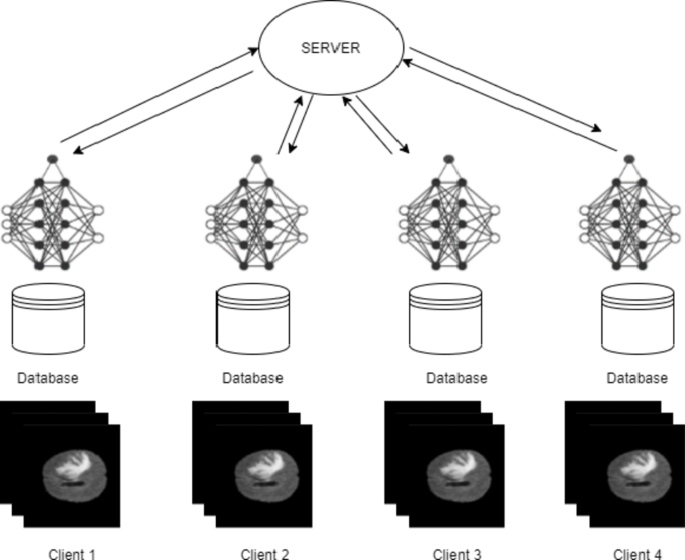
Model weights passed to the central server.