Data-driven total organic carbon prediction using feature selection methods incorporated in an automated machine learning framework

Figure 5 shows the computational framework for the proposed approach. The first process consists of cleaning the data (Data Cleanup), which aims to ensure the quality of the data set for carrying out the subsequent steps. With the completion of cleaning, this data is sent to the Feature Selection stage, which uses the BFS (Boruta Feature Selection), MI (Mutual Information), and RFE (Recursive Feature Elimination) techniques to choose the most relevant attributes. This data, now filtered, is destined for the Resource Processing phase, an important step for preparing the input information for the model. The processed resources are directed to the (Resource Building) stage, the Training Set. This training set will be used in model selection (Model Selection), where different algorithms are tested and adjusted in order to find the most appropriate one to solve the problem under study. This choice is made through hyperparameter optimization (Hyperparameter Optimization), so the model parameters are assigned to their ideal values. The models are evaluated by 5-fold cross-validation, which makes it possible to compare different solutions using a performance measure. The chosen and improved model is applied to the test set (Test Set) to make TOC (Total Organic Carbon) predictions. Finally, the predictions generated by the model are subjected to a Performance Analysis, in which quantitative measurements are employed to evaluate the model’s performance on the test set.

A detailed analysis was conducted to identify and correct both missing values and duplicates. By applying automated imputation techniques, missing and duplicate values could be eliminated, simultaneously guaranteeing the coherence and integrity of the underlying data. Data normalization was performed using the z-score standardization technique to make the attributes comparable to scales. This technique ensures that the mean is zero and the variance is one, improving training stability.

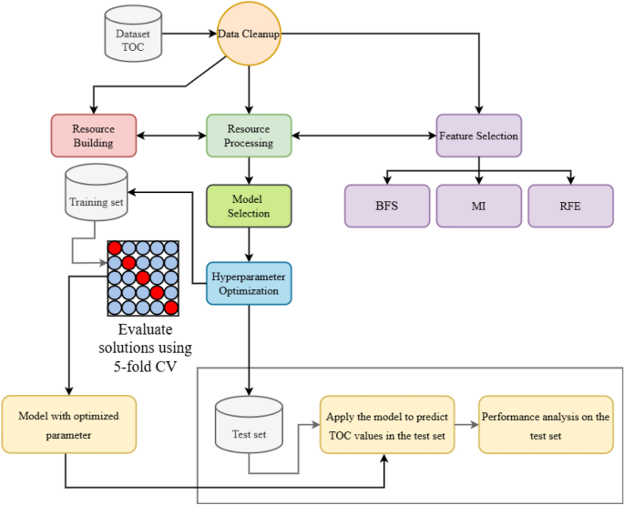
Framework for the proposed approach.

AutoGluon uses a grid search approach enhanced by meta-learning techniques, which adapts model selection based on the performance of previous models. This approach speeds up the process and increases the selection accuracy⁶⁰. The k-fold cross-validation technique was applied to evaluate the model’s performance and avoid overfitting. Stratified sampling techniques were used to maintain class distribution. This ensures unbiased results and accurate performance estimates. It is known that there is a potential bias generated by the shuffled training and testing divisions, leading each method to predict different test data and be trained on different training data. So this issue was taken into account. 200 independent runs were performed with different seeds, so the grid search employed, which uses Kfold, performed different divisions in the data, allowing a coherent analysis of the results. The models were evaluated using metrics appropriate to the TOC prediction, which is a regression problem. Table 4 shows the metrics used to assess the model’s performance.

Table 5 displays the models’ evaluation through the metrics RMSE, MSE, MAE, R² and R. XT was the method that obtained the best result in the test set, that is, on data not yet seen in the training process by the methods. The results show that some AutoML methods, such as XT and CatBoost, achieve good performance on the test set (data not seen by the methods) for the TOC prediction task. These findings suggest that these methods can be generalized well to new data.

In order to compare the effects of automated search parameters, a baseline model was implemented using default parameters, and its results were presented in Table 5. The parameter of the baseline XGB model according to Table 3 is 100 estimators (\(x_1\)), learning rate (\(x_2\)) equals 0.1, maximum tree depth equals 10 (\(x_3\)), child weight (\(x_4\)) set to 1, and subsamples (\(x_5\) and \(x_6\)) set to 1.0. As can be observed in Table 5, the models with parameter search and optimization achieved superior results in all metrics. This indicates that the parameter tuning process (whether manual or automatic) improves model performance by allowing it to be adapted to the characteristics of the data. This reinforces the importance of research in automated learning models to develop more robust and efficient strategies for determining model parameters.

Figure 6 shows a diagram of the families of models generated by AutoML, the model name, the score value, and the training time. The family that performed best was Greedy Weighted Ensemble_L2, which was generated through a greedy search in combination with methods to create a robust ensemble method. The parameters obtained in this family had a score equal to 0.2346 and a training time of 44.1 seconds. The two methods that obtained good results after the Greedy Weighted Ensemble were LGB and XT. Table 6 presents the best hyperparameters found during the training and the respective validation scores. Although GWE presents the best result in the set, this is not maintained in the test set, as shown in Table 5, likely because it is generated using a greedy search of the training and validation data, which can lead to overfitting.

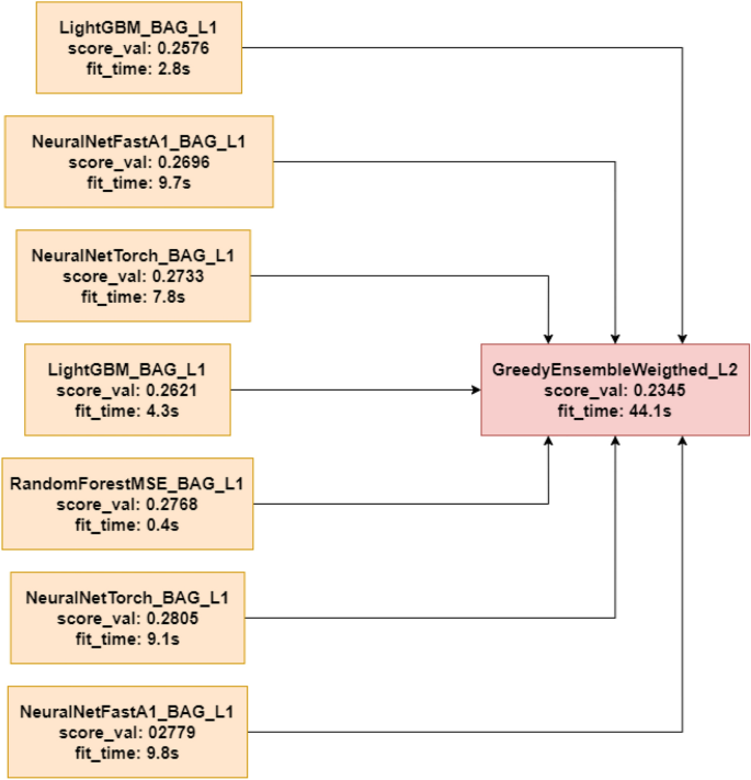
Greedy Weighted Ensemble model generated by AutoML.

Table 7 and Fig. 7 show the results incorporating feature selection approaches Boruta, Mutual Information (MI), and Recursive Feature Selection (RFE) into the developed models, considering 5 variables to Boruta, 3 to MI, and 3 to RFE. The assessment is based on root mean squared error (RMSE), mean squared error (MSE), mean absolute error (MAE), coefficient of determination (R²), and Pearson correlation coefficient (R). Additionally, the training time required for each model is also considered.

Across all the evaluated models, the incorporation of the Boruta feature selection method consistently yielded superior or comparable performance compared to MI and RFE. This is attributed to Boruta’s ability to effectively identify the most relevant features for TOC prediction while considering both their individual importance and interdependencies. The inclusion of a larger number of features, as selected by Boruta, provided the models with a more comprehensive representation of the underlying geological and petrophysical relationships influencing the TOC content.

In contrast, MI and RFE, with their tendency to select a smaller subset of features, resulted in models with reduced predictive accuracy. MI, based on information-theoretic principles, can not consider features with complex or non-linear relationships to TOC, while the iterative elimination process that is the basis of RFE can discard features that may contribute to the overall predictive power of the model. Consequently, models incorporating MI and RFE exhibited higher error values and lower correlation coefficients compared to those utilizing Boruta.

Furthermore, the XT (Extremely Randomized Trees) model emerged as a top performer across all feature selection methods, demonstrating low error values and high correlation coefficients. The robustness and effectiveness of the XT model in handling complex datasets with potentially non-linear relationships make it well-suited for TOC prediction tasks. CatBoost also exhibited strong performance, particularly with the Boruta feature set, highlighting the effectiveness of gradient boosting techniques in this domain.

Examining the final column of the table reveals that model XT achieved the fastest training times, with execution durations of 0.355 and 0.344 seconds, respectively. When considering recursive feature elimination (RFE) for feature selection, both models GWE and XT demonstrated promising results, with training times of 30.372 and 0.356 seconds, respectively. However, model XT emerged as demonstrably superior in terms of training efficiency.

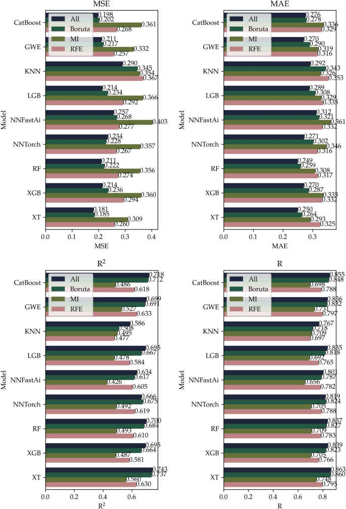
Comparison of performance metrics for reduced datasets. The original dataset has seven input features as described in Table 1, the Boruta feature selection yielded 5 features, and MI and RFE have 3 features each.

Feature selection analysis

A computational experiment was conducted to evaluate the effectiveness of different feature selection methods for TOC prediction using a dataset containing well-log measurements and corresponding TOC values. Feature selection can improve model performance and reduce training time in some cases. However, this task is challenging and there are many approaches in the literature. There are methods based on statistical tests, which use decision trees, among others. Three feature selection methods were compared: Boruta, Mutual Information (MI), and Recursive Feature Elimination (RFE). A total of 200 independent runs were performed for each feature selection method. In each realization, the data was shuffled, and each method was applied to select the most relevant variables. The dataset was then randomly divided into training and testing sets. The model was trained on the training set, and the testing set was used to calculate a performance metric. The MSE metric, described in Table 4, was used to compare the performance of the feature selection models.

Due to the randomization employed, each independent run yielded distinct results. A count indicator was used to track the variables selected in each run to identify the most relevant variables. If a variable was selected, the count returned 1; otherwise, it returned 0. If a variable was selected in all 200 runs, the count returned 200. Conversely, if a variable was selected in n runs, the count returned n. To simplify the decision-making process, the count was transformed into a percentage value, as presented in Table 8.

The variables obtained by the models differed due to their feature selection strategies. Table 2 shows that, of the seven variables, the most relevant for the Boruta method were acoustic time difference (AC), deep resistivity (RD), and uranium (U), thorium (Th), and potassium (K), appearing in 100% of the procedure’s runs. The input variables gamma radiation (GR) and shallow resistivity (RS) were listed 18.5% and 18% of the time, respectively. In this context, for the Boruta method, the GR and RS variables were disregarded, resulting in a set with five variables (AC, K, RD, TH, and U).

The results for Mutual Information (MI) yielded three relevant variables (AC, GR, RS), while the RD variable was discarded as it appeared in only 29% of the runs. The remaining variables were not selected by the strategy. Interestingly, MI excludes features like RD, TH, and U, which Boruta considered important. This difference highlights the varying approaches of these methods. The Recursive Feature Elimination (RFE) process yielded the variables AC, K, and U. The RD variable was disregarded as it appeared in only 9.5% of the independent runs.

Figure 8 shows a boxplot of the comparative performance measures using the reduced datasets with an XGB baseline model. The results indicate that the dataset produced by the Boruta method yielded the best performance, which is expected since the set has more variables, allowing the model to work with more formations and thus generate a model with greater accuracy and predictability. The proposed computational experiment shows that the Boruta method consistently outperformed the other methods, reducing the model complexity and the performance of ML models in this domain. However, it is important to note that the number of features selected by MI and RFE might be predefined or determined by the algorithm’s stopping criteria, which is limited to 3. In addition, for MI and RFE, the user-defined parameters can impact the number of features selected. Following are some facts that may justify Boruta having a better result: Boruta selects strong and weak relevant features by comparing feature importance with random features, ensuring robustness to irrelevant and redundant features. It works well with high/low-dimensional datasets and correlated features, which can hinder MI and RFE. It makes use of statistical tests to provide more reliable feature selection and can handle non-linear relationships more effectively. RFE and MI often miss weak but relevant features or fail to capture all information, while Boruta’s comprehensive approach tends to retain the most informative subset.

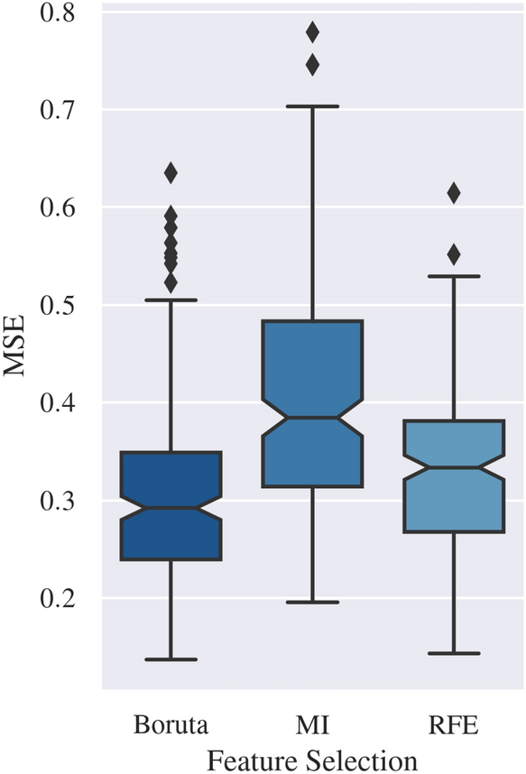
Comparative performance of features selection methods using the reduced datasets.

Each feature selection method used resulted in a different selection, some selected more, others less. It is important to evaluate the impact on the prediction as performed in the Subsection 3.2, in addition to using domain knowledge whenever possible^89,90, in this case the relationship between TOC and petrophysical features.

Feature importance analysis

Calculating the importance of features through permutation is a method verification tool that can be applied to supervised fitted models^71,91. Using this approach makes nonlinear models convenient. Feature importance is established by assessing the decrease in a model’s score when a single feature value is randomly shuffled. This procedure breaks the relationship between the feature and the target value, so the decrease in the model score is an indication of how much the model depends on the feature. For example, a feature importance of 0.02 indicates that the predictive performance decreased by 0.02 when the feature was randomly shuffled. The higher the score for a feature is, the more critical it is to model performance.

Table 9 shows the coefficients calculated by analyzing the importance of the variables. The same coefficients are displayed on a bar graph in Fig. 9. Observing Table 9 and Fig. 9, it is possible to extract crucial information about the importance of each feature in the model. A detailed analysis of feature importance seeks to interpret the crucial role of each input variable in the context of AutoML modeling, aiming to improve the precision of forecasting the total organic carbon (TOC) content in oil wells.

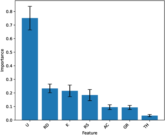
Bar chart of feature importance. The black line in the blue bars represents the standard deviation of the calculated importance, and the height of the bars represents the mean.

The characteristic uranium (U) takes center stage, which is important at 0.7393. This eminence is justified by the strong correlation between TOC content and uranium content resulting from the incorporation of this element during the deposition of organic matter. The role of U is so remarkable that one can anticipate a considerable influence on TOC predictions, revealing the distinctiveness of diagenesis. Its impact manifests not only as a direct indicator of TOC but also as a marker of specific geological environments that may harbor higher concentrations of hydrocarbons.

The deep resistivity (RD) importance is 0.2986. This robust relationship between actual density and TOC content provides a solid basis for the contribution of RD to the predictions. This characteristic reflects variations in wellbore properties, which, in turn, reflect the presence and distribution of organic matter. The extent to which the actual density varies may indicate the presence of zones with higher or lower organic matter content, directly impacting the TOC estimates.

The gamma ray (GR) plays a notable role, with an importance of 0.1468. This characteristic is important because of its ability to reflect not only natural gamma ray but also radioactive elements such as potassium, thorium, and uranium. These elements are often associated with organic matter and sediment minerals and thus have complex relationships with TOC levels.

The acoustic (AC) characteristic is highlighted with an importance of 0.1319. A direct connection between electrical conductivity and TOC content indicates its influence. The unique feature of electrical conductivity is its ability to provide information about the electrical properties of sediment at different depths. This makes it possible to identify zones where organic matter or conductive minerals are more significant. The link between shear wave velocity and TOC content provides insight into the relationships between wellbore mechanical properties and TOC.

The shallow resistivity (RS) has significant numerical importance, taking the value of 0.1115. The shear wave velocity (Rs) plays a key role in predicting TOC levels in oil wells, contributing to the understanding of the mechanical and structural properties of sediment. Its importance stems from the intricate relationship between shear wave velocity and the physical and geological properties of the well. The relationship between shear wave velocity and TOC content is associated with the porosity distribution and the presence of organic matter. In some cases, organic matter can fill the spaces between sediment grains, altering the propagation of shear waves. Therefore, variations in shear wave velocity may be indicative of changes in organic matter distribution and porosity. The shear wave velocity contributes to the direct estimation of TOC and provides information on wellbore architecture and variations in physical properties across depths.

The input variables thorium (Th) and potassium (K) exhibit similar importance, reinforcing their role in the analysis. TH reveals nuances with importance equal to 0.0507, indicating the presence of thorium in shale rich in organic matter. Similarly, potassium, with an importance of 0.04741, reveals the influence of potassium on well composition. Thorium and potassium traits are complementary in predicting TOC. The characteristic K (potassium) provides important information about the mineral composition of the sediment. Potassium is present in several minerals, and its concentration can vary depending on the type of rock and geological conditions. Although its contribution is relatively moderate, the presence of potassium in association with other radioactive elements, such as uranium and thorium, can influence the electrical properties and composition of the sediment. As a result, potassium (K) adds information about the complexity of the sedimentary environment. On the other hand, even though thorium has less prominent importance than other characteristics, it contributes to the understanding of the geological history of wells. Thorium is often associated with minerals that occur in sediments, and its presence may indicate certain sedimentary environments that favor the accumulation of organic matter. Therefore, including TH in the TOC prediction model allows us to capture nuances associated with specific geological contexts.

Discussion

This paper proposes an approach based on automated machine learning combined with feature selection approaches to investigate the prediction of total organic carbon (TOC) content. Considering the growing complexity of energy sources, the challenges in geochemistry and geophysics, and the exploration of energy resources in the energy transition era, this paper explored the potential of automated approaches to select the most suitable models and adjust their parameters to improve the accuracy of TOC predictions.

The proposed computational framework aimed to mitigate the limitations and bias associated with manual model selection and parameter setting approaches. The model consistently shows the potential to achieve reliable and consistent results, considering the complex interactions between models and underlying parameters. The automation of the TOC prediction process allowed the exploration of the search space, identifying the most promising combinations and, consequently, maximizing the predictive performance.

This approach is relevant because of the dynamic nature of the fields of geochemistry, geophysics and resource exploration^92,93,94. With technological advances and the increasing availability of data, implementing automated methods has become essential for optimizing informed decision-making. Furthermore, the approach contributes to biases and subjectivities by reducing human intervention in the selection and configuration phases.

Recent studies that have developed ML models for various versatile applications have reported that hyperparameter tuning is crucial for ensuring proper model performance⁹⁵. An effective fit can exploit the capabilities of simple models, resulting in competitive results. On the other hand, an inadequate fit can lead to a decline in the accuracy and robustness of models. An alternative to model tuning is the use of approaches that involve combining metaheuristics with ML models, resulting in hybrid models in which ML models benefit from automated search capabilities.

As the dataset size is limited, the application of complex models such as ensemble approaches increases the risk of overfitting, as the flexibility of these models makes them susceptible to capturing noise or irrelevant patterns in the data. Cross-validation helps estimate model performance (and reduces bias), but it may or may not prevent overfitting, especially if the data is limited or strongly unbalanced. In addition, early stopping, pruning, or limiting the number of ensemble trees can also further help reduce this risk by avoiding too many fittings. Also has the potential to enhance the dataset via data augmentation or synthetic data generation. The problem related to parameter search is formalized as an optimization problem in which grid search seeks to minimize metrics of interest, such as MSE (Mean Squared Error), while seeking the best combinations of hyperparameters^96,97. In some scenarios, variable selection can be easily built into models. In these cases, in addition to coding the hyperparameters, the solutions are designed to include binary arrays that turn on or off the variables that feed the ML model^48,98. More complex cases may involve sets of models, where the solution may indicate more than one learning model in a pipeline or linear combination strategy⁹⁹. Other studies, such as^100,101, show the need for the development of integrated artificial intelligence systems in the area of petroleum engineering and propose the use of techniques such as Principal Component Analysis to reduce the dimensionality of the data improving the performance and reduce the processing time of the artificial neural network used to predict porosity and permeability. This final approach can generate accurate but overly complex models. In these contexts, the goal is to maximize the performance of the model by increasing its precision while trying to simplify the models.

These objectives may conflict, leading to the formulation of a multicriteria problem, that is, a problem that encompasses multiple¹⁰² objectives. The solutions of interest, in this case, form a set of nondominated solutions known as the Pareto front. This front allows the decision maker to choose between more precise or simpler solutions, all equivalent to each other.

AutoML brings efficiency by automating model selection, tuning of hyperparameters, and feature engineering, but it also tends to be computationally intensive. Algorithms may vary in complexity and resource consumption based on their underlying functionality. As data sizes increase, consuming far more resources to train them, when training multiple models with a suite of algorithms, the process can be resource-intensive, often requiring CPU/GPU power and memory. In real-world situations, especially in the field, computational budgets are often limited, which can hinder detection. Running AutoML frameworks in those situations might require utilizing high-performance computers, cloud-based solutions, or optimized architectures, which can be avoided. Furthermore, some field applications require real-time predictions, making AutoML workflows inapplicable due to their generally slow work speed compared to the required decision time. The right use of this can be given for available future scenarios, which help in the later decisions. Therefore, a balanced approach is necessary, where the trade-offs between the power of AutoML and the practical constraints of the deployment environment are carefully considered.

The generalization of AutoML models to different geospatial and environmental conditions is a significant challenge. Although promising, AutoML frameworks usually need large, diverse datasets to train models and deliver decent performance on specific problems. In geoscientific use cases, we note that such data may be scarce, noisy, and specific to a region, resulting in models produced through AutoML not effectively generalizing to new, unknown environments without retraining or modification. In geoscience, professional expert knowledge is often lost in AutoML methods. Although AutoML may facilitate the efficiency of the model building process, it can simplify problems of a scientific nature by applying data-driven techniques without encompassing relevant domain knowledge. Hence, although AutoML is a very promising opportunity, it is crucial to bear these limitations in mind when applying it to geoscientific problems to ensure the results remain scientific and applicable to the real world problems.

As the problems faced in areas such as geochemistry and energy resource exploration become more complex, the interpretability of ML models has gained prominence. Interpretability is critical for understanding and trusting model results, especially in domains where decision-making is critical, such as the oil and gas industry. Models that predict total organic carbon (TOC) content in reservoirs can be black boxes, and their decisions can be difficult to understand and explain, making it difficult for domain experts to trust and practically adopt predictions. In these scenarios, interpretable models gain relevance, which can explain how a certain prediction was reached. One of the techniques to improve the interpretability of AutoML models is the analysis of the importance of variables, as developed in this study, which provides insights into which variables have the greatest influence on model decisions. Understanding and explaining model decisions is critical for ensuring expert confidence and the practical utility of predictions, and understanding and explaining model decisions is a key aspect of research and model development in these domains. However, in some cases, interpretable models can be oversimplified to favor interpretability, leading to a loss of performance in terms of predictive ability. Therefore, a balanced approach that considers both performance and interpretability is needed to address complex problems.

AutoML models can help experts predict total organic carbon (TOC) content, as they allow adaptation to different geological contexts. They can be trained on a variety of data from different geological contexts, allowing experts to use the learned knowledge in a wide range of scenarios. Determining TOC in core rocks can be a time-consuming process involving several steps. Interpreting these results is critical for understanding the hydrocarbon-generating potential of rock formations. Using ML models to support geologists results in greater agility in the analysis process because, as new data are collected, the ML models can be updated and refined easily. This allows experts to track changes in geological conditions and continually improve forecasts.