Analysis of space solar array arc images based on deep learning techniques

Solar array and the tested cells

Figure 2a shows pictures of a solar array sample of cells used in the experimental simulation. All dielectric–conductor junctions close to one interconnect area are insulated by tape to avoid spectral arcs between cells. The size of the sample cells is depicted in Fig. 2b²⁶. Detailed description of ground based simulation tests are discussed and presented in the works of Refs.^15,33. A circuit diagram for studying the arc behavior is shown in Fig. 3^15,34.

(a) Solar array sample, and (b) the size of the cells used in the test.

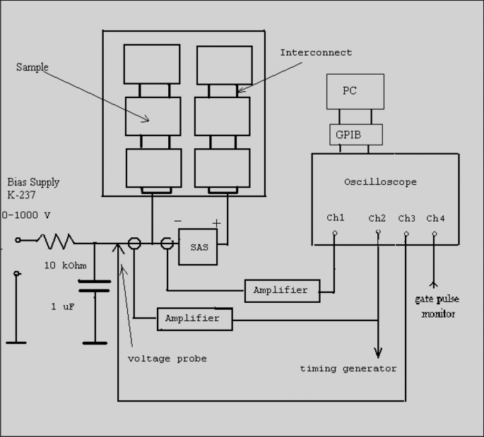
A schematic diagram of the circuit used for arc study.

Figure 4 illustrates the micrographic images of a sample of the cells in an array coupon shown in Fig. 3 after electrical discharges and arcs caused by the plasma impact. The arcing was recorded using a video camera at 30 frames per second to determine the arc site location. Arc sites are identified on interconnects and the cell edges³⁵. The figure displays the arcs observed at different positions of the cell surface: the cell edge, the interconnector with contamination, and the mid-cell. This is shown as Fig. 4a–c respectively. The images were captured by Prof. Boris Vayner at the Air Force Research Laboratory (AFRL)³⁵. The image in Fig. 4a shows arc discharge on the cell edge surface. These arcs can cause the ejection of metal atoms from the arc site resulting in contamination at the cell edges and spacecraft surfaces^20,29,35. Contaminations observed at the interconnected points near and at the cell edges are shown in Fig. 4b. The contamination is caused by the inverse gradient discharges located on triple junctions³⁵. For edge and contaminant surface, dimensions are about 5–8 mm. Figure 4c displays breakdown and micro-cracks formed on the cell coverglass. The scale shown for the breakdown area is 8495 µm (8.5 mm–1 cm). So, the number¹ refers to the diameter of a spot shown in the picture—approximately 1 cm. The thickness of the coverglass plus adhesive is about 150 µm (0.15 mm). The coverglass breakdown occurred under normal gradient discharge.

Images of (a) cell edge arc site, (b) interconnect contamination, and (c) mid -cell arc site.

The images shown in Figs. 4 were taken from a microscope in open air, consequently, the brightness is influenced by the reflection of light. The damaged areas observed in the images are not only caused by the arc itself but also by environmental conditions. That is why these images show more damaged and bright areas³⁵. These images are analyzed to understand the behavior and spatial variation in arc discharges on the cell and array surfaces.

Deep learning techniques

Dataset overview

In this section, it should be noted that, we could not obtain digital data or additional image data from the ground tests. Therefore, the dataset used for this study is limited. The dataset includes various types of solar cell defects, such as material degradation, micro cracks, arcing discharge, and shading issues³⁶. Not all defects in the training and validation dataset are caused solely by arcing. However, the validation dataset used to assess the model’s performance is focused specifically on arc-induced defects.

The dataset provides annotations for each image, indicating the defect probability (ranging from 0 to 1) and the type of solar module (either monocrystalline or polycrystalline) from which the solar cell is extracted. All images have been normalized for size and perspective, and any lens-induced distortions are corrected prior to extraction, ensuring consistency and accuracy in the dataset. A comprehensive dataset specifically designed for benchmarking the visual identification of defective solar cells in electroluminescence (EL) imagery is utilized in this research. The dataset consists of 2624 high-resolution grayscale images (300 × 300 pixels) of solar cells extracted from 44 different photovoltaic modules. The images include both functional and defective cells with varying degrees of degradation, which can adversely affect the power efficiency of solar modules^36,37.

Dataset usage

The dataset used in this study consists of high-resolution electromagnetic images of solar cells, categorized based on their condition. To facilitate its use, the dataset is organized into two main components:

1. 1.

   Images Directory All images are stored in the “images” directory. Each image represents a solar cell in a specific state (functioning or defective) and is provided in a standardized format (300 × 300 pixels, 8-bit grayscale).

2. 2.

   Annotations File The corresponding metadata and annotations for the images are stored in a CSV file named labels.csv. This file includes critical information such as:

   • Image Filename The name of the image file.

   • Probability The likelihood of defectiveness for each solar cell.

   • Type The specific defect type or classification label.

To streamline the dataset’s usage in Python-based workflows, the elpv_reader utility is available in the referenced repository. The utility enables users to efficiently load and preprocess the dataset with minimal effort^36,37,38. Below is an example of how to use this utility:

• from elpv_reader import load_dataset

• # Load images, defect probabilities, and types

• images, proba, types = load_dataset()

This code snippet automates the loading process and outputs three components:

• images A NumPy array containing the image data.

• proba A NumPy array of probabilities indicating defect likelihood.

• types A list of defect types or labels.

Requirements and licensing

• Dependencies The elpv_reader utility requires the installation of the following Python libraries:

• License The dataset is distributed under the Creative Commons Attribution-NonCommercial-ShareAlike 4.0 International License, which permits use for non-commercial purposes with proper attribution and requires sharing derivative works under the same license.

This structure ensures that the dataset is both accessible and user-friendly, facilitating its integration into various machine learning pipelines.

Data preprocessing and enhancement

The dataset is enhanced through preprocessing techniques, such as image contrast adjustment and feature highlighting, to improve the visibility of defect features and reduce misclassification risks associated with ambiguous labels. This ensures that the model is focused on visually evident defect patterns.

Image preprocessing and enhancement

Image preprocessing is a crucial step in any automated vision task. It involves preparing the raw image data in a way that enhances the performance of the model. We use a dataset of images of both healthy and defective solar panels to serve as the foundation for our model. Initial preprocessing involved resizing all images to a standard dimension of 224 × 224 pixels, followed by balancing the dataset using SMOTE (Synthetic Minority Oversampling Technique) to address class imbalances.

To improve the quality of the dataset and enhance defect visibility, we applied a series of preprocessing techniques before feeding the images into the model. These preprocessing steps are designed to ensure that defect features are more distinguishable, reducing the risk of misclassification due to ambiguous or low-contrast regions. The key preprocessing techniques used are as follows:

• Contrast enhancement Contrast limited adaptive histogram equalization (CLAHE) was employed to improve image contrast. CLAHE enhances local contrast, making subtle defect patterns more prominent while preventing over-amplification of noise. This technique ensures that critical defect details are more visible, aiding in better feature extraction during model training.

• Feature highlighting (edge enhancement—initial testing phase) During the preliminary analysis, Sobel edge detection filters were tested to emphasize vertical and diagonal edges, which could help in detecting defect patterns based on sharp intensity variations. However, after evaluating model performance, this step is not included in the final preprocessing pipeline as it does not significantly improve classification accuracy. The decision to omit this step is based on empirical results, which show that contrast enhancement alone is sufficient for highlighting defect features effectively. By implementing this preprocessing pipeline, we ensure that the model is focused on visually evident defect patterns, reducing the misclassification risks associated with ambiguous labels. The results demonstrate an improvement in model robustness by enhancing key defect features while maintaining the original structural details of the images.

Validation approach

The validation dataset is created to focus specifically on arc-induced defects, which are more visually distinct. While the broader dataset includes ambiguities in labeling, the validation process prioritized images with clear defect patterns to mitigate the influence of non-confident assessments.

It is crucial to carefully analyze as much data as possible, and we refine the dataset to ensure that the model can learn generalizable patterns.

Grayscale image equalization

This technique adjusts the contrast of images by spreading out the most frequent intensity values. By applying equalization, it assures that the images have a uniform distribution of intensity values, making it easier for the model to detect image defects.

Grid-based clutch creation

Using OpenCV, a grid with a size of (8 × 8 pixels) is applied to the images. This method helps in normalizing lighting conditions across the image, ensuring that different parts of the image are processed uniformly.

Handling class imbalance with oversampling

The dataset had an unequal number of images labeled as defective and non-defective, which could have led to a biased model. To address this, oversampling techniques are applied using sklearn’s oversampling functions. These generated additional samples for the minority class to balance the dataset and ensure that the model did not favor the majority class. To ensure that the data required for training are in optimal condition, preprocessing steps have been performed.

Libraries used

Several powerful libraries have been employed to streamline the process of building, training, and testing the model.

OpenCV (open source computer vision library)

OpenCV is an open-source computer vision and machine learning software library. It contains over 2500 optimized algorithms for a wide range of applications, including image processing and objects detection. In this study, OpenCV is used extensively for image preprocessing tasks such as grayscale equalization, grid-based processing, and also for visualization tasks concerning both two and three dimensional analysis.

NBLToolkits.nblot3d

This library is utilized to create three–dimensional (3D) visualizations. By using NBLToolkits.nblot3d, we are capable of generating 3D surface plots that provide a deeper understanding of the intensity distributions across the images. This helped in analyzing the patterns and structures that the model might be focusing on during its predictions.

Keras (with TensorFlow backend)

Keras is an open-source software library that provides a Python interface for artificial neural networks. Keras acts as an interface for the TensorFlow library. In this study, Keras is used to build and train the CNN model, leveraging TensorFlow’s powerful computation engine. The ability to easily define complex neural networks with minimal code makes Keras an ideal choice for deep learning mission.

Scikit-learn (sklearn)

Scikit-learn is a free software machine learning library for the Python programming language. It features various classification, regression, and clustering algorithms, including support vector machines, random forests, gradient boosting, and k-means. Scikit-learn (sklearn) is used to handle class imbalance through oversampling, a critical step in ensuring that the model learns to recognize both defective and non-defective cells equally well. Therefore, we applied an equalization function to each image to standardize the pixel intensity distribution. This step enhances the contrast in the images, making the defects more detectable by the model. OpenCV’s functionality is used to create a grid with a size of (8 × 8 pixels). This grid allowed us to apply local processing techniques that help in normalizing the lighting conditions across different parts of the image.

The dataset originally had an unequal distribution of the 0 and 1 labels, which could have biased the model (see Fig. 5). To address this, we applied oversampling technique using sklearn’s oversampling functionality. The left chart, in Fig. 5, represents the original dataset, which is unbalanced, meaning one class has significantly more samples than the other. This imbalance can negatively impact the model’s performance by biasing predictions toward the majority class. The right chart shows the dataset after applying a balancing technique, such as oversampling, undersampling, or synthetic data generation (e.g., SMOTE). Both classes have equal representation, which helps the model learn more effectively and make fairer predictions across all categories. The black arrow illustrates the transformation of the dataset before and after applying the balancing technique. This technique generates additional samples for the minority class, thereby balancing the dataset and improving the model’s ability to generalize. Examples of images with the enhanced versions are shown in Fig. 6.

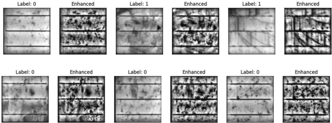
Samples of images and the improved version.