An enhanced moth flame optimization extreme learning machines hybrid model for predicting CO2 emissions

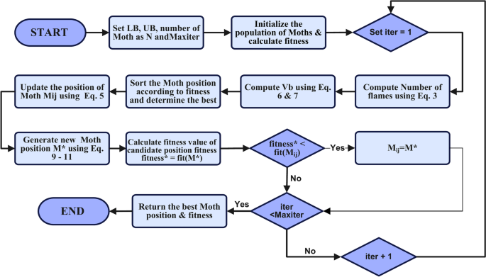
This section presents a comprehensive evaluation of the modified GMSMFO algorithm using the CEC2020 benchmark functions to assess its efficiency. The GMSMFO algorithm is compared against several MAs to demonstrate its rapid convergence capabilities and superior optimization performance. The analyses conducted include Convergence Plot, Box Plot, Friedman Rank (FR), Wilcoxon Sign Rank Test (WSRT), and Exploration vs. Exploitation Analysis. All evaluations utilize the CEC2020 benchmark functions, which consist of unimodal, multimodal, hybrid, and composite functions designed to test the efficacy of optimization techniques in solving complex real-world problems. The details of the test suite are provided in²⁶. GMSMFO is compared against four competitive optimizers introduced in the past decade: the Parrot Optimizer (PO)²⁷, Exponential Differential Optimizer (EDO)²⁸, Grey Wolf Optimizer (GWO)²⁹, and Moth-Flame Optimizer (MFO)²⁵. The specific parameter configurations for these optimizers are outlined in Table 1.

The experimental setup includes a maximum of 2000 iterations, 30 independent runs, and a population size of 30 for each optimizer.

CEC 2020

The experimental results of all competing algorithms on the CEC2020 benchmark functions for 30 and 50 dimensions are presented in Tables 2 and 3. These results include the average values (AVG) and standard deviations (STD) of the globally optimal values obtained for each benchmark function. The purpose of increasing the problem dimensions is to elevate the complexity of the optimization problems, thereby evaluating the performance of the optimizers under more challenging scenarios. A detailed analysis of the AVG values reveals that the proposed method achieves the smallest AVG in the majority of the benchmark functions, indicating its superior performance in handling increased problem complexity. From the average fitness presented in Table 2, GMSMFO achieved superior solutions in nine functions, including F1–F7, and F9–F10. In F8, the AVG fitness GWO surpassed that of GMSMFO slightly. This alludes to the fact that no single optimizer can be efficient for all problems. Furthermore, in the case of increased complexity, as seen in Table 3, GMSMFO maintained superior performance in F1–F7, and F9–F10. These functions span various types of optimization problem characteristics ranging from single-modal problems that evaluate the exploitation capability of the optimizer, multimodal problems that evaluate the exploration capability of an optimizer. The hybrid and composite problems evaluate the equilibrium between the exploitation and exploration capacity of an optimizer in handling complex problems. Notably, it can be established from both tables that GMSMFO demonstrated superior and efficient performance on the benchmark functions. This can be attributed to the improved exploration capacity of GMSMFO due to the incorporation of GM and SM strategies into the traditional MFO. These expanded the exploration capacity of GMSMFO and further balanced the exploration and exploitation phase.

Convergence curve and box plot analysis

Figures 4 and 5 show the convergence characteristic of the comparative algorithms and GMSMFO by plotting the average optimal result obtained by each optimizer against the maximum number of iterations. It can be observed that the GMSMFO gradually descended. This shows that GMSMFO is able to explore the search space efficiently and avoid local optimal solutions compared to other optimization algorithms characterized by a sharp drop and flat curve, which shows that they are unable to efficiently escape local optimal in complex problems. As seen in F1-F7 and F9-F10, GMSMFO efficiently converged towards a more optimal solution than other algorithms.

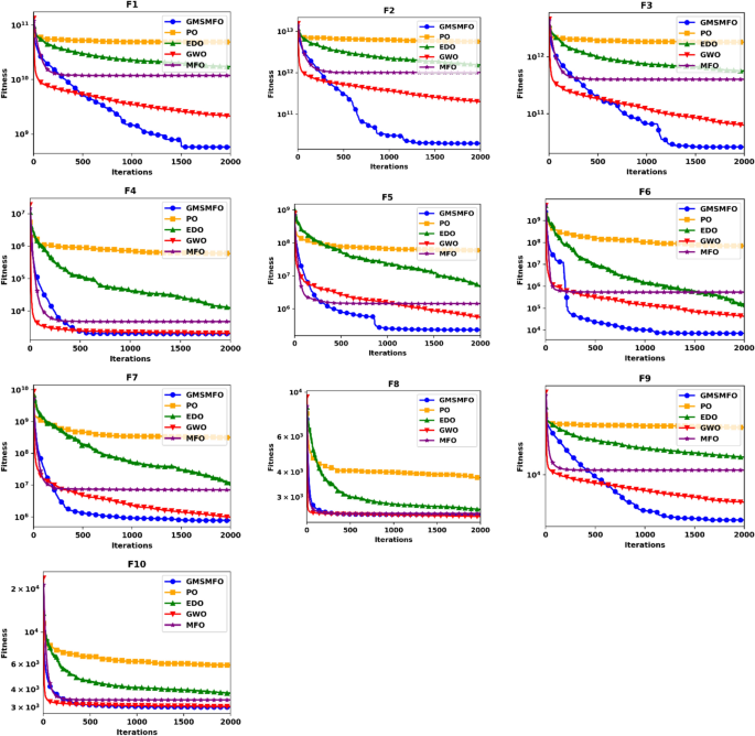
Convergence curve comparison of GMSMFO with other optimizer on CEC 2020 on 30-dimension.

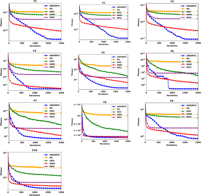
Convergence curve comparison of GMSMFO with other optimizer on CEC 2020 on 50-dimension.

Figures 6 and 7 represent the box plot analysis. The main rectangular box represents the interquartile range (IQR), which is the range between the first quartile (Q1, or 25th percentile) and the third quartile (Q3, or 75th percentile). It shows where the middle 50% of the data lies. A line within the box indicates the median (50th percentile) of the data, which is a measure of central tendency. This indicates the average performance for each algorithm. Lines or whiskers extending from the box represent the range of values. This gives a representation of the spread of the data. Points outside the whiskers are considered outliers, indicating extreme values that deviate from the general distribution, signified by the red “ + ” symbols. The box plot compares the performance of GMSMFO and the compared optimization algorithms based on the optimal results obtained by these optimizers over 30 independent runs. GMSMFO stands out as the most effective and consistent algorithm, with low medians and narrow interquartile ranges, suggesting it consistently yields low fitness values. This consistency indicates that GMSMFO provided reliable solutions across multiple runs. In contrast, PO has the largest IQR and several outliers in most cases, indicating high variability and a tendency to produce higher fitness values, making it less reliable. EDO and MFO perform moderately, with higher median values than GMSMFO and GWO, and exhibit more variability, though they are more stable than PO. Outliers are present for some algorithms, such as GWO and EDO, suggesting occasional deviations in performance. Finally, in the CEC2020 minimization problem, GMSMFO is the most efficient algorithm due to its lower mean values and consistent results, while PO’s high variability limit its effectiveness in achieving optimal solutions.

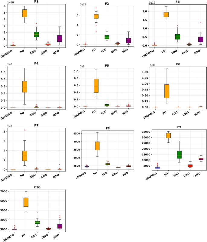
Box plot comparison of GMSMFO with other optimizer on CEC 2020 on 30-dimension.

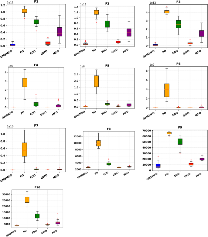
Box plot comparison of GMSMFO with other optimizer on CEC 2020 on 50-dimension.

Non-parametric test

The WSRT and FR, both widely used non-parametric statistical methods, are employed to conduct a comprehensive analysis of the experimental results. The WSRT is utilized to evaluate significant differences between paired samples, while the FR statistical method is used to determine whether there are significant differences between the performances of three or more related groups or methods. It is particularly useful when comparing methods across multiple conditions and datasets, where each method is evaluated under the same set of conditions. FR does not assume a specific distribution of the data, making it robust for ordinal or non-normally distributed data³⁰. Table 4 summarizes the results of the WSRT, performed on the experimental outcomes of all optimizers on the CEC2020 benchmark functions at 30 and 50 dimensions, with the results reported as Wilcoxon p-values. The p-values indicate that the GMSMFO method demonstrates significant superiority over EDO, GWO, and MFO, with values below the threshold at a significance level of α = 0.05. Additionally, Table 4 presents the ranks of the optimizers across all CEC2020 functions in both 30 and 50 dimensions, as determined by the FR, with the mean value of each optimizer denoted as the FR AVG. A general rank is subsequently assigned to each algorithm based on the FR AVG, providing an overall assessment of the optimizers’ performance. The results reveal that GMSMFO achieves the highest rank, thereby confirming its exceptional overall performance compared to other algorithms.

Exploration versus exploitation analysis

Exploration and exploitation are critical components of optimization algorithms, particularly those inspired by natural phenomena. Exploration involves searching widely across the solution space to uncover diverse potential solutions, thereby reducing the risk of the algorithm becoming trapped in local optima. This is especially beneficial in complex, multimodal landscapes. Conversely, exploitation focuses on intensively searching around regions that have already demonstrated promising results, enabling the algorithm to efficiently converge toward an optimal or near-optimal solution. Striking a proper balance between exploration and exploitation is essential for effective optimization. Excessive exploration can slow down convergence, while overly focusing on exploitation risks premature convergence to suboptimal solutions. As depicted in Fig. 8, the algorithm initially prioritizes exploration, enabling a broad sampling of the solution space, before transitioning to exploitation to refine the most promising regions. This dynamic adjustment ensures the algorithm achieves superior performance across diverse and complex problem domains due to the innovative incorporation of the GM and SM enhancement techniques.

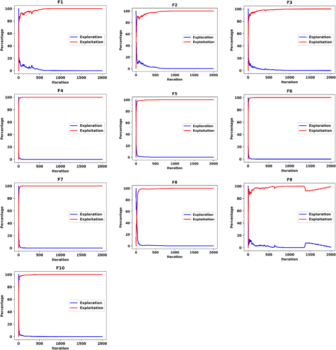
Exploration versus exploitation Plot of Gmsmfo.

Diversity analysis

Diversity is a fundamental concept in nature-inspired optimization algorithms, as it directly impacts the exploration–exploitation trade-off and the algorithm’s ability to converge to optimal solutions. Diversity refers to the distribution and spread of candidate solutions across the search space. Maintaining an appropriate level of diversity ensures that the algorithm avoids premature convergence to local optima while effectively exploring the search space to identify global optima. During the early stages of optimization, high diversity promotes exploration by enabling the algorithm to investigate various regions of the search space. As the optimization progresses, diversity typically decreases to facilitate exploitation, allowing the algorithm to refine solutions around promising areas. However, excessive loss of diversity leads to stagnation, where the population converges prematurely to suboptimal solutions, while excessively high diversity hinders convergence by preventing the algorithm from focusing on promising regions. Therefore, achieving a balance between exploration and exploitation through controlled diversity is essential for robust performance³¹. Two key metrics are utilized to quantify diversity: the population radius and the normalized diversity measure. The population radius, which represents the maximum Euclidean distance between any two individuals in the population, is mathematically defined in Eq. (17).

Here, \(\left| X \right|\) denotes the population size, \(D\) represents the dimensionality of the problem space, and \({X}_{i,t}\) corresponds to the position of the \(i\)-th individual in the \(t\)-th dimension. This metric captures the spatial extent of the population, offering a measure of how widely the individuals are dispersed across the search space. Complementing the population radius, the normalized diversity \({D}^{N}\) is computed using Eq. (18)

where \(\overline{X}_{t}\) represents the center of the population in the \(t\)-th dimension. This normalized measure evaluates the spread of individuals relative to the population center while accounting for the scaling effect of the population radius. As a result, it enables a standardized assessment of diversity across different stages of the optimization process and varying problem dimensions.

As illustrated in Fig. 9, the traditional MFO exhibits a very high level of diversity during the initial stages of the optimization process compared to the GMSMFO. This heightened diversity in MFO is attributed to its high stochastic nature and lack of appropriate strategy to transition to localized search mechanisms during the early iterations. However, as the optimization progresses, GMSMFO demonstrates a notable improvement in maintaining balanced diversity during the intermediate stages of the search process. This behavior is attributed to the incorporation of advanced mechanisms such as the SM and GM, which enhance population diversity while ensuring a smoother transition from exploration to exploitation. The results presented in Tables 2 and 3 further corroborate this observation, showing that GMSMFO effectively converges the population towards regions containing optimal solutions more efficiently than MFO. In contrast, the traditional MFO struggles to aggregate the population around the optimal solution region despite exhibiting higher diversity in the initial stages. This limitation arises due to the absence of robust local escaping techniques and an inadequate balance between exploration and exploitation. As a result, MFO tends to lose diversity prematurely, leading to stagnation and suboptimal convergence. On the other hand, GMSMFO’s ability to maintain refined and moderate diversity throughout the optimization process ensures a more comprehensive exploration of the search space while gradually focusing on promising regions, thereby achieving superior solution quality and convergence behavior performance.

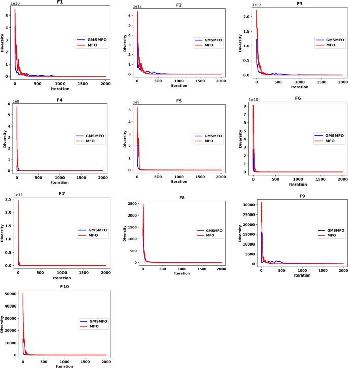
Diversity plot of GMSMFO.

Time complexity

The computational time results presented in Table 5 provide a detailed comparison of the efficiency of GMSMFO and compared optimizers when applied to the CEC2020 benchmark suite in a 30-dimensional search space. The average computation time in seconds presented in Table 5 reveals that GMSMFO consistently demonstrates lower computation times compared to MFO across most benchmark functions (F1–F10). This reduction in runtime is attributed to the structural enhancements in GMSMFO, which eliminate excessive loops and iterations over the population for each operation performed on the population, Algorithm 1. For instance, in traditional MFO, operations such as sorting the flame population and updating moth positions involve multiple nested loops that iterate over the entire population, leading to increased computational overhead. In contrast, GMSMFO streamlines these processes by incorporating efficient mechanisms, such as vectorized operations and a single loop, which minimize redundant computations and enhance overall execution speed. For example, in functions F4, characterized by higher complexity and multimodality, GMSMFO achieves significantly lower computation times than MFO (e.g., 43.037 s vs. 40.819 s for F4). This improvement is particularly noteworthy given that GMSMFO also incorporates additional operations, which could have otherwise increased its runtime. Eliminating excessive loops in GMSMFO reduces computational overhead and ensures that the algorithm maintains a balance between exploration and exploitation without compromising efficiency.

PO exhibits the least computation times across all functions except F4. The results highlight the effectiveness of GMSMFO’s design improvements in reducing computational time while maintaining competitive solution quality. By eliminating redundant loops and optimizing population-based operations, GMSMFO achieves faster convergence and improved scalability, making it a more efficient choice for solving complex optimization problems compared to traditional MFO. These findings emphasize the importance of algorithmic refinements in enhancing computational efficiency, particularly in scenarios where runtime is a critical constraint.

Evaluation of GMSMFO-ELM model on CO₂ prediction

Evaluation metrics

This study included five assessment metrics: coefficient of determination (R²), Root Mean Squared Error (RMSE), Normalized Root Mean Squared Error (NRMSE), Mean Absolute Error (MAE), and Mean Square Error (MSE) to evaluate the performance of the proposed model. The mathematical formulations are given in Eqs. (19–23)

These metrics collectively provide insights into the accuracy and reliability of a predictive model. Where \({y}_{i}=\) actual values, \(\hat{y}_{i} =\) predicted values, \(\overline{y} =\) mean of actual values, \(n=\) number of observations.

The R² measures the proportion of variance in the actual data explained by the model, with higher values indicating better fit. However, R² alone does not account for overfitting or biases, necessitating complementary metrics for a complete evaluation. The RMSE quantifies the standard deviation of residuals, emphasizing more significant errors between the actual and predicted values due to its squared nature, and is critical for assessing precision in predictions. Similarly, the MSE evaluates the average squared differences between the predicted and actual values, highlighting deviations between them. The MAE calculates the average absolute difference between predictions and observations, treating all errors equally and providing robustness against outliers. Lastly, the NRMSE normalizes RMSE relative to the mean of actual values, enabling scale-independent comparisons across datasets. Lower values of RMSE, MSE, MAE, and NRMSE, alongside a high R², signify superior model performance.

In this research, these metrics collectively ensure the model’s result reliability. High R² values confirm the model’s predictive power, while low RMSE, MSE, MAE, and NRMSE values demonstrate precision and generalizability. Such rigorous evaluation is essential as accurate CO₂ predictions support policy formulation, climate mitigation strategies, and sustainable development planning. By leveraging these metrics, the study validates the GMSMFO-ELM model’s effectiveness, ensuring its applicability in diverse scenarios and reinforcing its potential as a robust tool for addressing environmental challenges.

Data

The datasets utilized for CO₂ emissions and other input variables in this study were obtained from credible sources, including the World Bank (WB)³², Our World in Data (OWD)³³, and established literature by Solt³⁴. The data encompasses quarterly data in the United States over the period 1970 to 2022. To maintain data integrity and ensure consistency, comprehensive preprocessing was undertaken. This involved transforming the data into their logarithmic form and to reduce the impact of variables with large magnitudes on others in a dataset, standardization was applied. Such rigorous preprocessing steps are critical in preparing the datasets for accurate and reliable analysis. Detailed metrics are presented in Table 6, while Figs. 10, 11, and 12 illustrate the distributions, trends, and correlation matrix, offering deeper insights into the data structure.

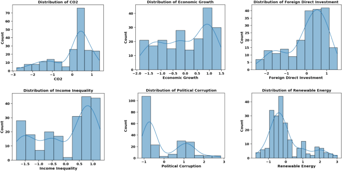
Distribution of features.

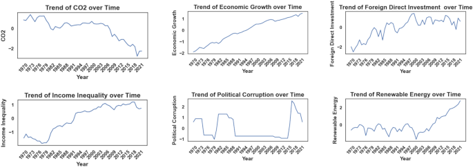
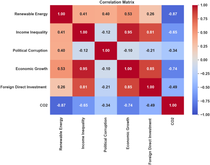
CO₂ prediction results

In this section of the study, the performance of the proposed GMSMFO-ELM model is evaluated and compared against algorithm-based ELM and traditional ELM approaches across various evaluation metrics during both training and testing phases. The parameter settings outlined in Table 1 are consistently applied to all algorithms, with the number of iterations set to 100. The search boundaries for the weights and biases of the ELM are within the range of − 10 to 10, and the population size for each optimizer is fixed at 30 search agents. The error metric utilized for fine-tuning the weights and biases of the ELM model, as defined in Eq. (12), is MSE. Additionally, the dataset is split into training and testing subsets in a 70:30 ratio to evaluate the model’s performance comprehensively.

In Table 7, the performance of GMSMFO-ELM is benchmarked against other optimizer-based models and the traditional ELM. During the training phase, GMSMFO-ELM achieved an R² value of 0.9758, the highest among all models, indicating a predictive accuracy of 97.58%. This superior predictive capability is attributed to the enhanced diversification capabilities provided by GM, enabling the model to avoid local optima effectively. In contrast, models like EDO-ELM and PO-ELM recorded lower R² values of 0.9333 and 0.9317, respectively, reflecting their limited ability to capture data variance and potential susceptibility to underfitting. The RMSE metric further underscores GMSMFO-ELM’s accuracy, with a training RMSE of 0.0378, significantly outperforming EDO-ELM and GWO-ELM. This lower RMSE indicates reduced prediction errors, demonstrating that GMSMFO-ELM delivers more precise predictions within the training set. This enhancement is attributed to GMSMFO’s balance between exploration and exploitation through SM strategy. Moreover, GMSMFO-ELM exhibited the lowest MSE of 0.001432, underscoring its minimal average squared error and validating the effectiveness of GM in achieving an optimal solution. Comparatively, MFO-ELM and PO-ELM yielded higher MSE values of 0.002837 and 0.004043, respectively, highlighting their less precise parameter tuning processes. The MAE results further affirm GMSMFO-ELM’s superior predictive accuracy, with a value of 0.0297, the lowest among all models. This indicates that GMSMFO-ELM consistently produces minimal absolute prediction errors, maintaining small deviations from actual values. In contrast, EDO-ELM and PO-ELM showed higher MAE values of 0.0505 and 0.0514, respectively, suggesting their greater susceptibility to errors. Lastly, GMSMFO-ELM achieved the lowest NRMSE value of 0.1575 during training, reflecting its adaptability across the dataset and superior generalization performance. Models such as GWO-ELM and PO-ELM reported higher NRMSE values of 0.1983 and 0.2706, respectively, underscoring GMSMFO-ELM’s ability to deliver superior performance across multiple evaluation metrics.

In the testing phase, as detailed in Table 8, GMSMFO-ELM demonstrated its continued superiority over other models. The R² value for GMSMFO-ELM on the test set was 0.9545, indicating that it maintained a high level of accuracy even on unseen data. This strong R² suggests that GMSMFO-ELM is highly resistant to overfitting and exhibits excellent generalization capabilities. In comparison, models such as EDO-ELM and PO-ELM showed significantly lower R² values, reflecting poorer generalization performance. The RMSE of GMSMFO-ELM on the test set was 0.0501, the lowest among all models, highlighting its minimal prediction error and robust performance. Models like GWO-ELM and traditional ELM, with RMSE values of 0.0624 and 0.0830, respectively, underscore the advantage of GM in enabling GMSMFO to achieve more accurate global solutions. Additionally, GMSMFO-ELM’s MSE was the lowest at 0.002514, emphasizing its ability to minimize average prediction errors on unseen data. In contrast, PO-ELM and ELM exhibited higher MSE values of 0.006707 and 0.006893, respectively, depicting their higher susceptibility to errors.

The MAE metric further validated GMSMFO-ELM’s accuracy, with the lowest value of 0.0397 on the test set, signifying minimal absolute prediction errors. Comparatively, models like EDO-ELM and MFO-ELM recorded higher MAE values of 0.0688 and 0.0477, respectively, indicating their greater susceptibility to deviations. Similarly, GMSMFO-ELM achieved the lowest NRMSE value of 0.2258, substantially outperforming other models, such as EDO-ELM and PO-ELM. This low NRMSE underscores GMSMFO-ELM’s exceptional ability to generalize effectively across the data. The findings reveal that GMSMFO-ELM consistently outperforms traditional MFO and other optimization algorithms during both the training and testing phases. The integration of GM and SM enhances the optimization capabilities of the MFO algorithm, enabling GMSMFO to achieve better global solutions while minimizing prediction errors. This effective balance between exploration and exploitation allows GMSMFO-ELM to deliver highly accurate CO₂ predictions, establishing it as a robust and reliable model for addressing complex optimization problems. The implications of these evaluation metrics are significant for the GMSMFO-ELM model’s application in CO₂ prediction. High R² values confirm the model’s ability to capture complex emission patterns, while low RMSE, MSE, MAE, and NRMSE values ensure precise and reliable predictions with low errors,

The plot in Fig. 13 illustrates the progression of MSE over 100 iterations for various ELM models optimized using different algorithms, including GMSMFO-ELM, PO-ELM, EDO-ELM, GWO-ELM, and MFO-ELM. Among these models, the GMSMFO-ELM consistently achieves the lowest MSE values throughout the iterations. It demonstrates a steep decline in MSE early in the optimization process, followed by continuous improvements, reflecting effective convergence and superior optimization compared to the other models. This rapid reduction and lower final MSE highlight the strong exploration capabilities of GMSMFO, enabling it to escape local minima and achieve more optimal solutions. In contrast, the PO-ELM model exhibits a steady reduction in MSE initially but stabilizes at a higher MSE level than GMSMFO-ELM, indicating its limitations in achieving the same level of optimization. Similarly, the EDO-ELM and GWO-ELM models show gradual declines in MSE but plateau at higher values, suggesting a less effective balance between exploration and exploitation in optimizing the ELM for this task. The MFO-ELM model maintains the highest MSE values throughout the iterations, displaying minimal improvement and highlighting its limited optimization capability compared to GMSMFO. Overall, the GMSMFO-ELM model distinguishes itself with rapid convergence and significantly lower MSE, underscoring the effectiveness of the GM and SM in enhancing the exploration abilities of the MFO algorithm. This superior performance demonstrates GMSMFO’s ability to optimize the ELM for CO₂ prediction tasks effectively.

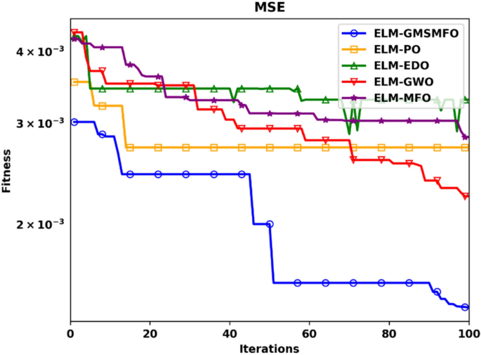
MSE convergence of GMSMFO-ELM and compared models.

Figure 14 illustrates the prediction performance of the GMSMFO-ELM model compared to other models on both training and testing datasets. The plot includes three key elements: the actual values (represented by a black line with stars), the predicted values from each model, and the absolute error (depicted by a pink line). The x-axis corresponds to the data samples, while the left y-axis represents the observed and predicted values. The plot is divided into a shaded green area, which highlights the test set, and a white shaded area representing the training set. The predictions from the GMSMFO-ELM model closely follow the actual values, indicating its capability to effectively capture the underlying trends in the data. However, some fluctuations between the predicted and actual values are evident and are highlighted by the absolute error curve (pink line) plotted against the right y-axis. While the error values reveal minor deviations between predictions and actual values, they generally fall within a relatively narrow range compared to other models. This suggests that although GMSMFO-ELM is highly accurate, minor prediction errors may arise due to the complexity of the test data or residual noise in the model’s fit. The plot demonstrates that GMSMFO-ELM excels at capturing the true trends in the data, with most errors being minimal. The consistent alignment between the model’s predictions and the actual values, along with the relatively small error range, underscores the model’s robustness and reliability for CO₂ prediction tasks. These results highlight the effectiveness of integrating GM and SM, which enhances the exploration and fine-tuning capabilities of the model, ultimately improving its accuracy.

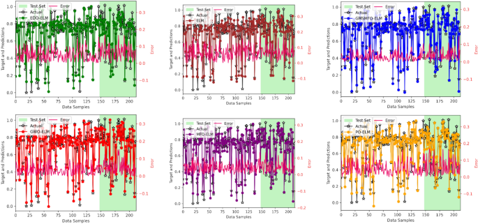
Actual an predicted values of GMSMFO-ELM and compared models.

In this study, the performance of the GMSMFO-ELM model for CO₂ prediction was evaluated and compared to other optimization-based ELM variants and the base ELM model. The scatter plots in Fig. 15 depict the relationship between predicted and actual values for both training and testing datasets, with R² values providing a quantitative measure of accuracy. GMSMFO-ELM exhibited the highest predictive accuracy, achieving R² values of 0.976 for training, 0.954 for testing, and a combined total R² of 0.965. The scatter plot for GMSMFO-ELM shows data points closely aligning with the y = x line, signifying minimal error and a strong correlation between predicted and actual values. This superior performance highlights the effectiveness of the GM and SM enhancement, which has significantly improved the exploration capabilities of MFO, resulting in a well-tuned ELM model for CO₂ prediction. In comparison, EDO-ELM demonstrated weaker performance, with R² values of 0.933 for training, 0.882 for testing, and a total R² of 0.908. Its scatter plot reveals a more dispersed pattern around the y = x line, particularly in the testing set, indicating its limitations in capturing data variability. The base ELM model performed the least, with R² values of 0.895 for training, 0.875 for testing, and a total R² of 0.885, showing significant deviation from the y = x line. This suggests overfitting during training and poor generalization to unseen data. GWO-ELM and MFO-ELM performed comparatively better, with R² values of 0.962 and 0.930 for GWO-ELM and 0.952 and 0.939 for MFO-ELM, respectively. However, their scatter plots revealed slightly more variance around the y = x line compared to GMSMFO-ELM. GMSMFO-ELM’s superior alignment along the y = x line and its highest R² values across both datasets affirm its robustness and enhanced generalization capabilities. These results demonstrate that the integration of GM and SM into GMSMFO effectively improves the original MFO algorithm, making GMSMFO-ELM the most reliable and accurate model for CO₂ prediction among the methods tested. This study underscores the potential of GM to enhance optimization algorithms by improving diversity and SM to balance exploration and exploitation, leading to more accurate and generalizable predictive models.

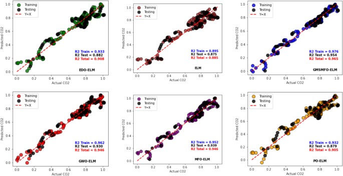
Scatter plot of GMSMFO-ELM and compared models.

Permutation importance score

In the GMSMFO-ELM model, permutation importance scores were calculated using MSE to evaluate each variable’s impact on CO₂ emissions prediction. The permutation importance score is a model-independent metric that quantifies the influence of each feature by shuffling its values and observing the resulting change in the model’s error. Specifically, if the MSE increases significantly after shuffling a particular variable, it indicates that the variable plays a crucial role in the model’s predictive accuracy. Conversely, if the error changes minimally, the variable likely has less influence on the model’s outcome. The use of MSE as the measure for permutation importance allows for a clear assessment of how much each variable contributes to reducing prediction error. The permutation importance analysis conducted for the GMSMFO-ELM model highlights the relative significance of each variable in predicting CO₂ emissions, as seen in Fig. 16. Economic growth (EG) emerged as the most influential variable, which aligns with existing literature that links higher GDP per capita with a great impact on CO₂ emissions^35,36. The high importance of EG in the model indicates its substantial impact on emissions prediction. Following EG, foreign direct investment (FDI) showed considerable importance. FDI can lead to the establishment of energy-intensive industries, potentially increasing emissions. However, FDI’s environmental impact varies, as some investments support clean technology transfer, reducing emissions^37,38. Renewable energy (RE) is also influential. Renewable energy directly mitigates emissions by reducing reliance on fossil fuels. The importance of RE in the model underscores the positive impact of clean energy adoption, aligning with numerous studies promoting renewables as crucial for emission reduction^36,39. Income inequality (IQ) also affects CO₂ emissions, as socioeconomic disparities can lead to unsustainable resource use among both affluent and impoverished segments⁴⁰. Finally, Political corruption had the least impact on the model’s predictive performance. The GMSMFO-ELM Permutation importance scores are particularly valuable because they provide insights into the model’s reliance on each variable without altering the model’s structure. By identifying the most critical features, these scores contribute to validating the model’s assumptions and enhancing its interpretability, providing a deeper insight into the factors influencing emissions predictions in the GMSMFO-ELM model. The scores underscore the complex interplay of economic, social, and political factors impacting CO₂ emissions in the U.S. from 1970 to 2022.

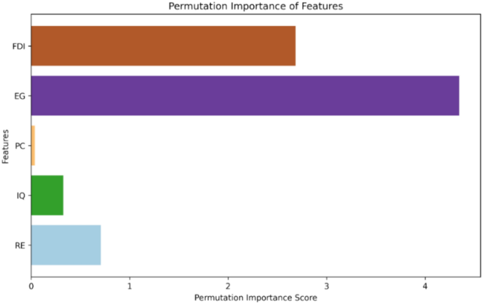
Permutation importance of features of GMSMFO-ELM.