An efficient bearing fault detection strategy based on a hybrid machine learning technique

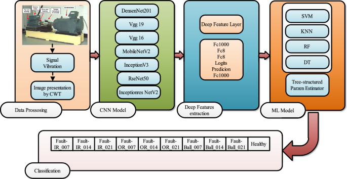
Time–frequency image representations are then classified using features acquired from seven different famous convolutional neural network models. Initial attempts to implement the DL algorithms are performed on a laptop with 16 GB of RAM and an Intel Core i5 CPU. In the training phase, the parameters affecting the accuracy of the various machine learning techniques are determined using the TPE method. These hyperparameters do not change during training as well as testing of the model on the test data set. The features extracted from each model are classified using four different ML techniques, including support vector machines, decision trees, k-nearest neighbors, and random forests. The confusion matrices for the given classification results are shown in Fig. 4 below. Apart from the confusion matrices, other measures that are derived from these matrices are computed and shown for the assessment of performance. These metrics served as numerical evaluations of the classification performance of the applied machine learning method.

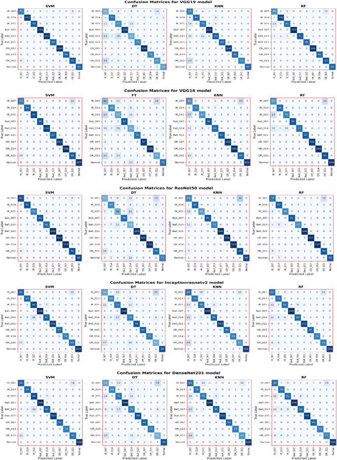
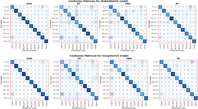
Confusion matrix results.

The confusion matrices in Fig. 4 for the various models (VGG16, MobileNetV2, Inception V3, and DenseNet201) show distinct patterns of performance. The SVM model shows very good performance in most classes, especially in Ball_007, Ball_021, and Normal, where it only misclassifies a few instances of IR_007. The DT (Decision Tree) model performs well in classes like Ball_007 and Ball_021 but is poor in both Ball_014 and Normal. The KNN model performs quite well although it misclassifies IR_007 and Normal, while making a few mistakes in Ball_007 and Ball_021. Random Forest (RF) performs very well in all categories, but Ball_007 and Normal had the best results, while IR_007 and IR_021 had some errors. Most importantly, in the majority of the cases, SVM and KNN proved to be more effective than DT and RF on the other side, RF is stronger in stability and gives higher generalization as it has fewer errors of IR_007 and Ball_021. In general, these results reveal the dichotomy of accuracy and generalization, with SVM and KNN making fewer mistakes within certain categories, whilst RF exhibits greater resilience across all fault types and balance performance.

Table 6 demonstrates the effectiveness of machine learning methods, employing hyperparameters determined by the TPE for features produced from each CNN model. Comparative analysis shows that ResNet50 is the most accurate model, while SVM is identified as the most stable classification model. In particular, the structure of Res-Net50 with SVM allows achieving a high classification accuracy of 95.51%. This result is achieved through feature extraction from images using ResNet50 and using SVM for classification. The accuracy, sensitivity, and specificity for the Res-Net50-SVM structure are 0.9554, 0.9537, and 0.9542, respectively, while the MAE, RMSE, and R2 values are 0.21384, 1.1629, and 0.8374, respectively.

Figure 5 shows the ROC curve of Resnet50 for four different machine learning classifiers: SVM, KNN, RF, and DT. The AUC-ROC values of every classifier are also provided below. The ROC curve shows how well a classifier is performing, and the area under the ROC curve is a performance measure. The value of AUC-ROC also signifies a better classifier, and a higher value of it is preferred. In this figure, it can be seen that the AUC-ROC of the SVM model is 0.99, meaning the model is exceptionally accurate in predicting the outcome of a patient; the RF model has 0.98; the KNN has 0.94; and DT has 0.78, representing the accuracy of the model in predicting the outcome of a patient.

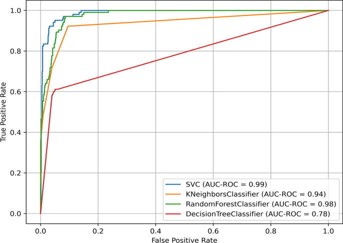
ROC curves of the Resnet50 structure.

Figure 5 is the ROC curve of four classifiers, including SVC, KNeighborsClassifier, RandomForestClassifier, and DecisionTreeClassifier, which maps the TPR against the FPR. The AUC pairs these rates at different classification levels, illustrating the trade-off between them. The ideal curve for a good classifier will lie as near as possible to the top-left corner of the plot—a high TPR with a low FPR. In this figure, it can be seen that the SVM classifier has the highest value of AUC-ROC, with its curve closely located to the upper left corner of the graph. Other classifiers, such as RandomForestClassifier, yield an AUC-ROC of 0.98, and KNeighborsClassifier has a 0.94 AUC-ROC, while DecisionTreeClassifier has an AUC-ROC score of 0.78. Based on the results of this experiment, SVM is shown to be the best classifier among the three. The ROC curves for both the Random Forest (RF) and K-Nearest Neighbors (KNN) classifiers show good performance, which is evident from the curves being very close to the upper left-hand corner of the plot. Nonetheless, the ROC curve of the Decision Tree (DT) classifier is less effective and has a lower value of AUC-ROC. In general, it is evident from Fig. 5 above that the Support Vector Machine (SVM) has the highest AUC-ROC score, meaning that it is the best classifier for this task and is followed by the RF and KNN classifiers. However, the DT classifier is relatively poor when compared with the other models of classification.

Figure 6 presents the precision-recall curve of Resnet50 for four classifiers: SVM, KNN, RF, and DT. The classification performance of each model is presented using the AUC-PR, the area under the curve of precision-recall. The AUC-PR value is higher if the model has better classification ability; the SVM model is 0.90, Random Forest 0.84, KNN 0.80, and Decision Tree 0.62.

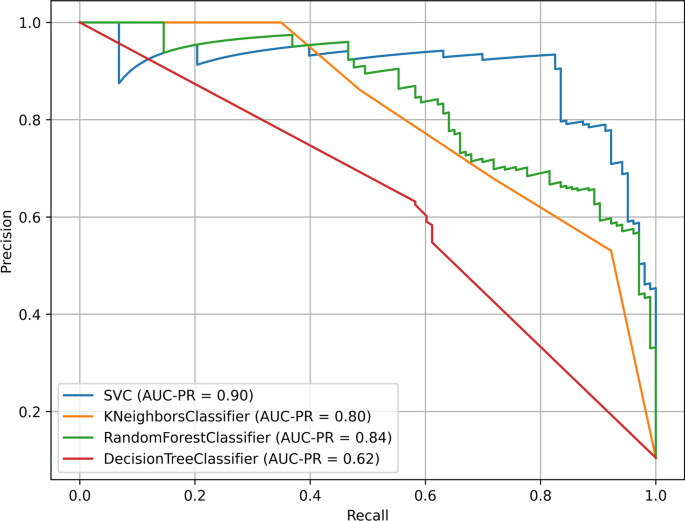
Precision-recall of the Resnet50 structure.

The aperture is an approach that is used to represent the trade-off between precision and recall, where we have the precision-recall (PR) curve. Precision denotes the ratio of the true positive predictions to the total number of positive predictions made, while recall shows the number of actual positive cases correctly categorized amidst all the positive predictions made. From the PR curve in Fig. 6, the classifier with the highest precision and recall is the SVM classifier and is followed by the Random Forest and KNN, with the Decision Tree performing poorly on this classification task.

As it can be seen in Fig. 6, the precision-recall curve of the SVM classifier shows the highest precision for most of the recall values, indicating that the classifier performs the best for this task. The precision-recall curves for the RF and KNN are also good, but the precision-recall curve for the DT is slightly lower since DT has low precision for most recall values. From Fig. 5, it is clear that the SVM classifier is the most accurate classifier for this task, followed by the RF and KNN. The DT is not as good as the other classifiers. In summary, both Figs. 5 and 6 continually point out SVM as the best classifier for the given task, and it performs better in both ROC and precision-recall analyses. As for the rest of the algorithms, RF and KNN show much higher results than DT. These findings are useful in identifying the relative strengths of classifiers and, hence, in choosing the most appropriate model for a given classification task.

As shown in Fig. 7, the average accuracy scores of different machine learning classes, including Random Forest (RF), Support Vector Machine (SVM), K-Nearest Neighbors (KNN), and Decision Tree (DT), trained by a dataset using the ResNet50 structure are presented. The plots illustrate how training and validation accuracy evolve as the training set size increases, with accuracy values ranging from 0 to 1, where 1 represents perfect classification.

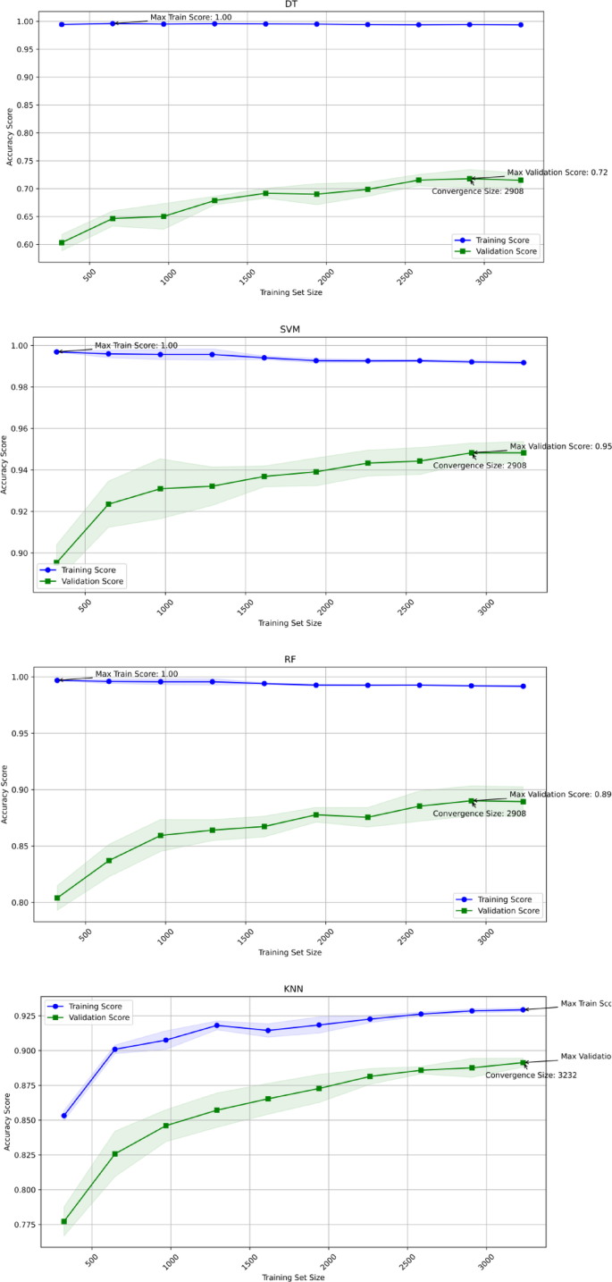
The average accuracy score of a training set of ResNet-50.

As we can see from this figure, the RF model can reach a maximum training accuracy of 0.99 when the training size is 3142, and the validation score oscillates around 0.92. The SVM classifier also achieves a good training accuracy of 0.99 and a validation score of 0.95 when the training set of 2195 is used, which shows better generalization. The KNN model has the maximum training accuracy of 0.94, but the validation accuracy converges to 0.84, meaning that the model is still good. Nevertheless, the DT model, which has received a nearly perfect training accuracy of 0.99, has many problems with overfitting. It is to be noted that the validation accuracy of the model begins at approximately 0.6 and increases to only 0.81. The difference between training and validating accuracy shows that, although the DT model achieves high accuracy on the training set, its performance is significantly lower on new data. However, the SVM and RF models are much better balanced between training and validation performance, with small differences between the scores obtained, which means better generalization. However, the KNN algorithm is only average, with training and validation scores climbing as the dataset size increases with the final validation accuracy of 0.91 at convergence. In general, the results indicate that all the models yield good training accuracy, but the SVM and RF classifiers are the most generalized, followed by KNN, while DT may have a little problem with overfitting.

The method was tested on a more complex dataset containing different operating conditions like loads and motor speeds (1797, 1772, 1750, and 1730 rpm) where torque values changed from 0 to 3 HP. There were 4 primary defects along with their respective fault diameters (inner race, outer race, and ball defects) of 0.007 inches. Although there were some limitations due to computation expense, the results showed very powerful multi-model classification. In particular, SVM yielded 100 percent accuracy, while KNN and RF models each reached 99% accuracy. DT showed a 92% accuracy which indicates the ability of the method to classify fault conditions. It can be concluded that the proposed methods work for various fault types and operating conditions and can therefore guarantee dependable diagnosis of faults.

The primary computational complexity arises during the search and selection phase, where the optimal CNN architecture and hyperparameters are determined using TPE. This phase involves computational overhead due to extensive model evaluations and optimizations. However, once the optimal configuration is identified, the final deployed model-ResNet-50 combined with SVM operates with significantly reduced complexity. ResNet-50, a pre-trained deep learning model, efficiently extracts features, while SVM ensures robust classification with lower computational cost compared to fully end-to-end deep learning models. This trade-off allows the proposed approach to maintain high detection accuracy while remaining computationally efficient for practical applications.

Comparison with some previous studies

Table 7 presents a comparison between the actual study and some previous works. In contrast to prior studies that have achieved higher rates, this method brings a new approach by combining CWT with feature extraction and hyperparameter tuning using TPE. This hybrid method not only increases classification performance but also improves generalization across multiple classes. Based on the model results, it is rated to be very robust because it achieves a classification accuracy of 95.51%. Because of this, the proposed framework can be considered more useful and dependable than models that focus on achieving the highest accuracy, thus making the methodology more applicable to real-world problems. In fact, accuracy alone does not fully determine the superiority of a method.

Study outcomes and limitations

The results of the proposed approach show that the accuracy rate is 95.51% when the multimodal feature extraction techniques are used in DL models like ResNet50-SVM. To validate its generalizability for different operating conditions, the proposed approach is tested on datasets covering different types of fault conditions including, inner race, outer race, and ball faults. A combination of different operational conditions including motor speeds 1797, 1772, 1750 and 1730 rpm, and torque levels ranging from 0 to 3 HP are employed to validate the robustness of the models. Despite its high accuracy, the real-time applicability of the approach remains untested, which may present challenges in practical deployment. Additionally, while the model demonstrates strong performance within the experimental dataset, variations among different rotating machines could affect its applicability, leading to inconsistent success rates across industrial environments.

According the obtained results and study limitations, future works will focus on evaluating the computational burden of the ResNet50-SVM hybrid model and comparing its performance with lightweight alternatives such as MobileNetV2. Additionally, efforts will be made to estimate the processing time required for data analysis to determine the feasibility of the proposed method for real-time applications. Further research will also involve applying these models to more complex datasets that encompass a wider range of operational parameters, including varying motor speeds and loads.