A three-stage machine learning and inference approach for educational data
With the collection of student-level characteristics, there exists a range of machine learning algorithms that could make decent predictions based on the past performance of a student. For example, Cortez and Silva3 applied a basic neural network, support vector machine, random forest, etc., to achieve a classification accuracy as high as approximately 90% in binary outcome and a root-mean-square error as low as 1.32 in the Portuguese data. However, machine learning algorithms alone are not capable of making statistical inferences regarding the unknown population relationship between a factor of interest (e.g., parents’ education) and the academic outcome of the student. Therefore, this work adopts a three-stage pipeline that aims to provide a generic approach to making inferences in educational data.
To put it simply, in the first stage, LASSO logistic regression, random forest, and LASSO regression are implemented on an expanded feature set to obtain a short list of explanatory variables of interest. In the second stage, for each explanatory variable, a post-double-selection process as introduced in41 is conducted to obtain a set of potential control variables. The last stage uses linear regression and IVs to draw a statistical and potential causal inference. The paper also demonstrates how recent advances in econometrics could be used to perform sensitivity analysis on the estimated linear regression coefficients under omitted variable bias. Figure 4 outlines the three-stage approach.
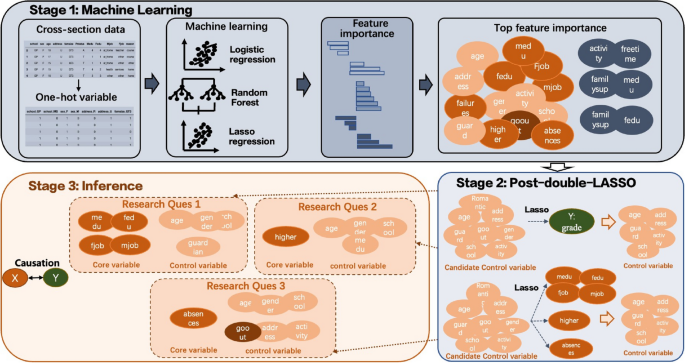
Three-stage machine learning and inference approach.
On the one hand, the purpose of machine learning is to make predictions, so the smallest error (e.g., mean squared error) is chosen to improve the prediction performance. However, our purpose is not only to predict but also to explain the causal relationships of variables in reality. Machine learning algorithms can flexibly choose a functional form to fit the data to obtain better predictions. Therefore, the more features there are in the machine learning model, the more accurately the results can be predicted. In this way, machine learning algorithms are designed to become increasingly complex. The prediction method of machine learning does not consider the consistency and unbiased characteristics of the estimated coefficients. It simply chooses to trade bias for smaller loss to improve prediction performance.
Stage 1: machine learning
The target of the first stage is to examine all variables and select a subset of explanatory variables for further inspection in the next two stages. Note that this manuscript differs from3 in two ways. First, this work considers the interactions among variables and their squares, while in3, only variables in their original forms are inspected, which leads to moderating and diminishing effects being overlooked in the analysis. Second, our choice of machine learning algorithms differs from theirs, as this paper utilizes methods that perform well in dimension reduction instead of prediction accuracy.
That said, this manuscript first expands the set of variables in their original forms by including meaningful interactions of two variables with the student’s age and the squares of the original variables. Note that the one-hot version of the categorical variables is used in the interaction.
Table 3 shows all interactions included. The first seven rows examine whether factors such as the choice of guardian, parenting style, and financial support provider further enhance students’ academic outcomes relative to the time they spend studying. The second row builds on this analysis by exploring the potential moderating effect of students’ health status. Rows 8 to 10 focus on the influence of family education as a moderating factor on students’ academic performance. Rows 11 to 13 investigate the impact of different extracurricular activities, not only in terms of their type but also the amount of time students dedicate to each. Finally, the last four rows analyze the potential heterogeneous effects of engaging in romantic relationships, considering students’ demographic backgrounds and time allocation patterns.
To reduce the bias that may arise due to similar optimization procedures, the study implements the LASSO logistic model, random forest, and LASSO regression to compress the enriched feature space. Specifically, the LASSO logistic model adds an l1 penalty term to the usual logistic objective function that involves the sigmoid transformation. The random forest considers Gini impurity, which measures the relative frequency of misclassification. These two methods view the outcome variable (i.e., course grade) as categorical. And to determine the robustness of the results, the grades are converted into classes in two ways—(i) binary: P/F for passing and failure, and (ii) multiclass: A (≥ 16), B (≥ 14), C (≥ 12), D (≥ 10), and E (< 10).
While other classification algorithms are widely employed in various fields, for our purposes—balancing dimension reduction, interpretability, and effective information utilization—LASSO logistic regression and random forests are the most suitable choices. For example, decision trees could be considered, but their feature selection mechanism is inherently incorporated into random forests, contributing little additional information to the ensemble. Similarly, support vector machines may offer an alternative, but they lack an intuitive framework for assessing the relative importance of selected features. Finally, neural networks typically require substantially larger datasets than ours and lack a transparent method for determining variable importance, making them unsuitable for our proposed methodology.
In contrast, LASSO regression treats course grades as numerical, and its loss function is the mean squared error with an l1 penalty attached. A similar popular alternative to LASSO, designed for numerical outcome variables, is ridge regression. However, in our context, ridge regression is less suitable because it merely shrinks the coefficients of unimportant variables toward zero without eliminating them entirely. As a result, it does not effectively reduce the feature space, which is a critical requirement for the second and third stages of the proposed pipeline.
Table 4 shows the top ten features with the highest importance determined by each algorithm. In general, this first-stage result provides guidance on which variables could potentially be influential explanatory variables when minimal knowledge is available. In this paper, three variables that are highlighted multiple times by different algorithms are intentionally selected from the table to conduct further analysis in the following two stages. The reason for this choice lies in the different types of endogeneity that one might encounter in a generic educational dataset, which places the pipeline in a more generic setting.
Specifically, the three sets of variables and their related research questions are as follows.
-
1.
Between the parents’ occupation and educational background, which factor is more important?
-
2.
Does the aspiration to pursue a higher degree lead to higher course grades?
-
3.
Does class absence substantially worsen grades?
Stage 2: post-double-LASSO for the control variables
To draw statistical inferences and even to make causal statements, one should properly address different aspects of endogeneity embedded in each explanatory variable. One of the major threats is omitted variable bias, and a classical challenge in the big data era is that a large set of candidate control variables is available, but there is minimal prior knowledge on which subset of the control variables should be used. Mathematically, there are two competing forces. On the one hand, if any confounding factor is missing from the model, the linear regression estimators will be biased and inconsistent. On the other hand, if too many controls are included, the correlation among them will cause a close-to-perfect-multicollinearity situation, which undermines the stability of the point estimates.
The conventional approach is to report regression results for several different sets of controls and show that the parameter of interest is insensitive to changes in the set of control variables. This strategy relies on existing theories to offer guidance about which variables to use. However, when the setup of the problem is new, variable selection is usually arbitrary. Inspired by the rapid development and popularity of various dimension reduction methods in machine learning, in a seminal paper, Belloni et al.41 proposed a post-double-selection procedure to select the set of control variables at the discretion of the model in lieu of arbitrary handpicking. While many previous studies have utilized this intuitive idea of using machine learning to select control variables before running a linear regression, their approaches usually suffer from two sources of bias. The first bias is due to imperfect variable selection—i.e., variables at the margin of the choice are retained or dropped arbitrarily. The second is the single-selection bias that arises if the selection is conducted only once with the outcome variable on the left-hand side of the model.
Belloni et al.41 provided rigorous mathematical proofs along with simulation studies to demon strate the severity of the aforementioned two types of bias and demonstrate the validity of a so-called post-double-selection procedure. In essence, the procedure is to perform variable selection twice using an appropriate dimension reduction algorithm. When LASSO is the chosen method, it is called post-double-LASSO. The procedure works in the following way. First, this study runs a LASSO of y on a set of candidate control variables to select a subset of predictors for y. Then, the research runs LASSO for the explanatory variable of interest, d, on the set of candidate control variables to select a set of predictors for d. Last, a linear regression of y on d is implemented and take the union of the sets of the regressors selected in the two LASSO runs; the inference is simply the usual Heteroskedasticity robust inference in this regression.
One could make sense of this procedure from the perspective of omitted variable bias. In linear regression, omitted variable bias occurs when a confounder—i.e., a variable that is correlated with both y and d—is excluded from the model. From this standpoint, the first LASSO filters regressors that are associated with y, and the second LASSO retains variables that are related to d. The union of the two sets, therefore, should include all potential confounders given the data at hand.
Table 5 shows the variables that are selected by the post-double-LASSO procedure. Many variables are commonly selected, for example, the address of a student (rural vs. urban), who is the guardian, whether the student is engaged in a romantic relationship, the reason for the course choice, etc. Due to the collinearity among variables, in the three illustrative linear regressions in the next section, a subset of the post-double-LASSO variables will be used as the control variables.
Stage 3: inference based on OLS regression
In this section, this paper will conduct three sets of linear regressions to answer the questions posted at the end of Section “Stage 1: machine learning”. The main challenge is the endogeneity embedded in each explanatory variable, ranging from unobserved confounders to reverse causality. Along the way, the research will demonstrate how the control variables selected in the second stage help in modeling the regressions and how sensitivity analysis could be employed to enhance the credibility of the regression coefficients under omitted variable bias.
Case # 1. Parents’ occupation and educational level
In theory, a professional occupation and a decent educational degree of the parents would help to build study environment conducive to better academic outcomes for the student.
To gauge which factor is more influential, it is tempting to place all one-hot indicators of occupation type and educational level on the right-hand side of the linear regression. Nevertheless, collinearity among the variables would impede stable point estimates. That said, the question is handled in two steps: first, this paper regresses the course grades on the occupation type and educational level for each part of the parents. The most significant factor from each parent is retained and combined in a follow-up regression to see which combination of mother-father and occupation-education plays the most important role in boosting the course performance of the student.
The first-step regression takes the following form:
$$Grade3_{i} = \beta_{0} + \beta_{1} job_{i} + \beta_{2} edu_{i} + \gamma Controls_{i} + \varepsilon_{i} ,$$
(1)
where Grade3i is the course grade of student i in the 3rd observational period; jobi is a categorical variable indicating four types of parental occupations—teacher, health industry, service sector, and staying at home—and other; edui is also categorical, indicating five types of educational level, 0 (none), 1 (primary education (up to 4th grade)), 2 (5th to 9th grade), 3 (secondary education) and 4 (higher education); and Controlsi stands for a collection of control variables informed by the results in stage 2.
The chief threat to the regression method above is omitted variable bias due to unobserved student ability. It has been established in many existing studies that parental profession and educational background are positively correlated with the ability of the children. Hence, the omission of student ability would inflate the point estimate.
The traditional approach is to either use fixed effects in a panel regression to absorb the impact of ability or include a proxy for student ability. Due to data availability, neither is feasible in the UCI dataset. Notably, while the course grades in the preceding observational periods could shed light on student ability, they should not be used as the proxy because they are also the outcomes of the explanatory variables, making them bad controls, as suggested in42.
Recent advances in econometrics provide an alternative—the sensitivity analysis introduced in43. The idea is to add a hypothetical variable to the linear regression that is contrived to have an impact at different levels of magnitude than the existing variables. By varying the variable to be compared, one can see how the point estimate and its t-statistics would change under different scenarios. In this way, despite not controlling for the confounders, one is able to tell whether, in the worst case, the error in the point estimates of the core explanatory variables would become insignificantly different from zero.
Tables 6 and 7 show the estimated coefficients in Eq. (1) under different specifications of the control variables. Note that while the results in stage 2 suggest a larger set of control variables, the research experiments on the subsets and demonstrate the robustness of the regression coefficients when the subset of controls is both reflective and of a reasonably low variance inflation factor (VIF).
The main results of interest are g3M and g3P—the course grades in the 3rd observational period for Math and Portuguese. For robustness, the estimates are shown for these two subjects in the first two periods. Note that in all regressions, observations where parental education is below elementary school are excluded, as they account for less than 1% of the entire sample and can be regarded as outliers.
Using an occupation of other as the benchmark, while in some scenarios (e.g., the mother’s job being health care and the father’s being teacher) the estimates are significantly positive, their effects become indistinguishable from zero when indicators for the educational levels are added and the full set of control variables are included.
In contrast, educational level exhibits a more stable impact on course grades for both parents and both subjects. It is shown that compared to an elementary school degree, if either of the parents has a higher degree, the course grades of their children are on average approximately 1.5 points higher than others. Notably, the impact of a higher degree of the mother is larger in Math than in Portuguese, despite there being no substantial heterogeneity in the impact of the father’s degree.
Figures 5 and 6 demonstrate the stability of the estimates of the parents’ educational levels under different hypothetical scenarios. Consistent with the qualitative argument, the inclusion of a hypothetical variable that has an impact at different levels of magnitude than existing variables would lead to a lower point estimate in terms of absolute value. In all setups, the t-statistics are greater than the critical value of 1.96.
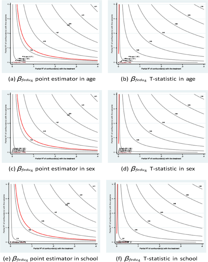
Sensitivity analysis of fedu4 in Eq. (1) of case #1 in Math.
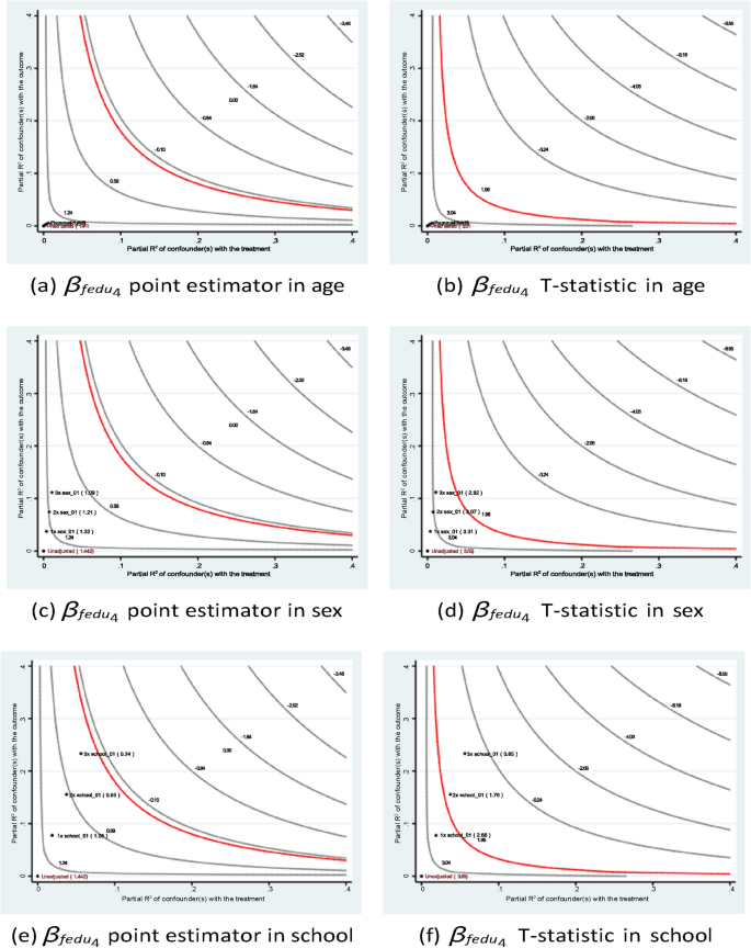
Sensitivity analysis of fedu4 in Eq. (1) of case #1 in Portuguese.
These preliminary results on the relative importance of occupation and educational background motivate the following regression to further investigate the contribution of the parents:
$$Grade3_{i} = \beta_{0} + \beta_{1} medu_{i} + \beta_{2} fedu_{i} + \gamma Controls_{i} + \varepsilon_{i} ,$$
(2)
where the explanatory variables are medui and fedui, with the same definitions as in Eq. (1).
Equation (2) shares the same endogeneity concerns with the previous regression model in terms of unobserved student ability. Therefore, this paper includes the same set of control variables and sensitivity analyses to demonstrate the validity of the estimated coefficients. Additionally, note that students who have at least one parent with an educational level below elementary school are dropped from the estimation to obtain results comparable to those in Eq. (1).
Table 8 exhibits the regression results under different specifications of the controls and for different outcomes of interest. It turns out that the mother having a higher degree is significantly positive in all regression settings, and the father’s educational contribution now becomes negligible. Moreover, the magnitude of the impact is similar to the results of Eq. (1), where the impact is higher for Math and lower for Portuguese.
The sensitivity analysis results shown in Figs. 7 and 8 confirm the stability of the estimates of the father’s education. In short, the research founds a similar pattern of academic contributions from the parents’ educational backgrounds to those found in many existing studies. For instance, Özyıldırım44 conducted a meta-analysis of 37 studies involving over 45,000 students to examine the impact of parental involvement on students’ academic motivation. The analysis found that parental involvement has a small but statistically significant overall effect on academic motivation. These findings suggest that policy interventions aimed at improving educational accessibility not only benefit current students but may also positively influence future generations.
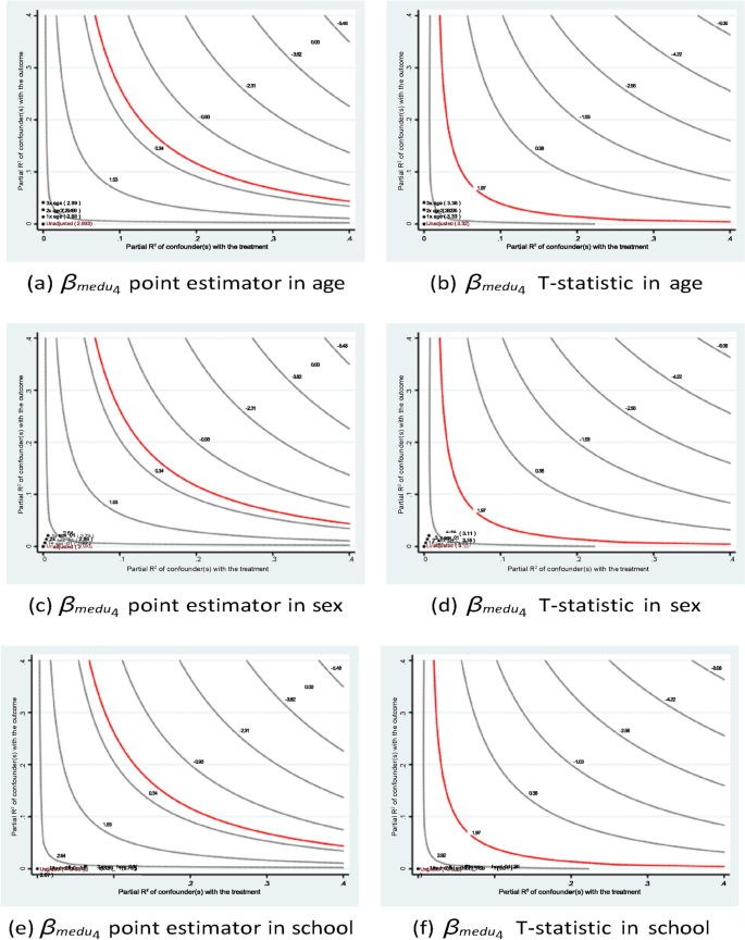
Sensitivity analysis of medu4 in Eq. (1) of case #1 in Math.
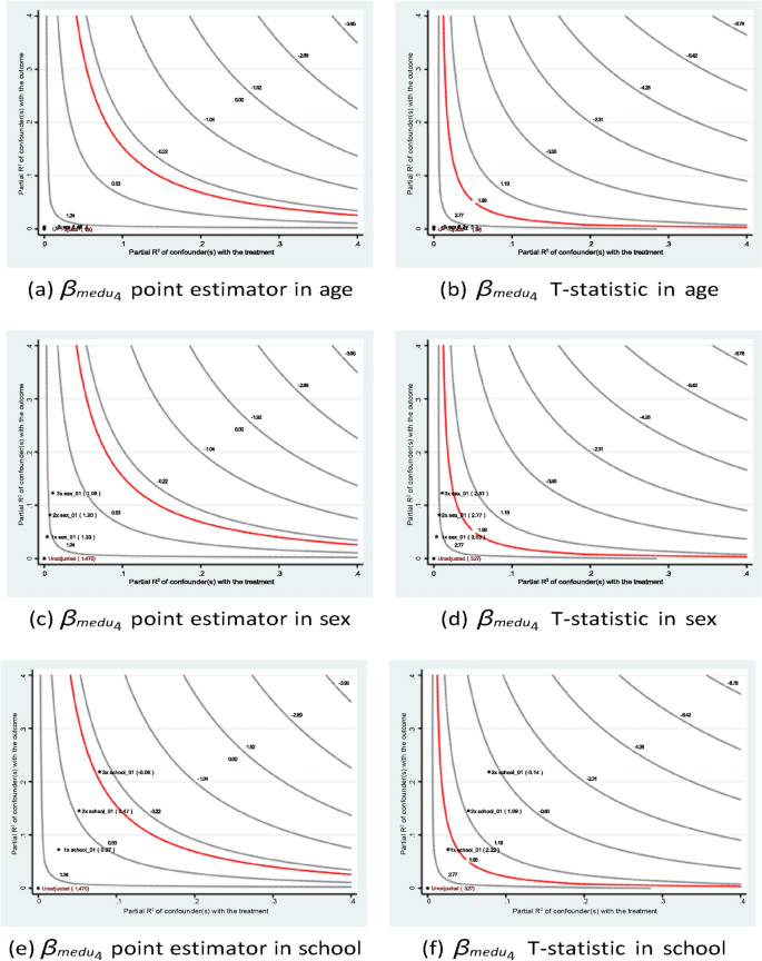
Sensitivity analysis of medu4 in Eq. (1) of case #1 in Portuguese.
However, technically, my work differs by adopting a model-driven approach in which the explanatory variables are first found by machine learning algorithms and the corresponding control variables are selected as a result of post-double-LASSO.
Case # 2. Intention of obtaining a higher degree
A considerable proportion of the students in the UCI dataset declared in the survey their intention to pursue a higher degree after graduation. In this section, this paper investigates whether this aspiration leads to better course performance. The following linear regression model is estimated:
$$Grade{3}_{i} = \beta_{0} + \beta_{{1}} Higher_{i} + \gamma Controls_{i} + \varepsilon_{i} ,$$
(3)
where Higheri is a binary value taking the value 1 if the student answers yes in the survey and Controlsi stands for a subset of the control variables, as suggested by the second stage.
There are two major empirical threats to Eq. (3). First, similar to the previous case, the unobserved student ability is a confounding factor that is excluded from the model. Presumably, a student with greater talent would prefer additional education and obtain a better grade, which would cause an upward bias when estimating β1. Second, the description of the dataset does not make the timing of the survey clear; hence, it is unknown whether the indicated intention of further education was declared before or after the students knew their latest grade. In the latter scenario, there would be reverse causality from Grade3i to Higheri.
Unfortunately, due to the lack of a valid IV for Higheri, this research can only evaluate, to some extent, the association between the two variables. To do so, the same sensitivity analysis is applied to gauge the stability of βˆ1 when hypothetical variables are added into the regression.
Table 9 shows the estimated coefficients of Eq. (3) and Fig. 9 as well as Fig. 10 demonstrate the robustness of the strong positive estimates of βˆ1 when hypothetical variables of different levels of impact are added to the regression. Due to collinearity among the candidate control variables, this paper includes only a subset of the variables that are reflective and have substantial variation as suggested by post-double-LASSO. It is shown that the students who intend to pursue a higher degree on average score three more points in Math and two more in Portuguese than other students. The magnitude is high given that most grades cluster between 8 and 15.
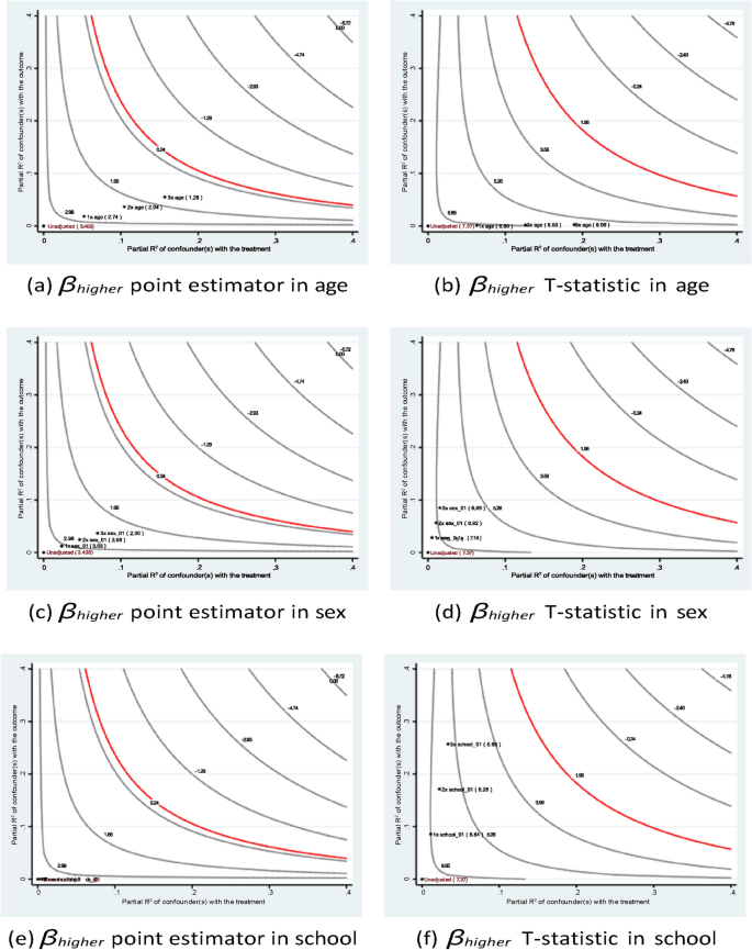
Sensitivity analysis of higher in Eq. (3) of case #2 in Math.
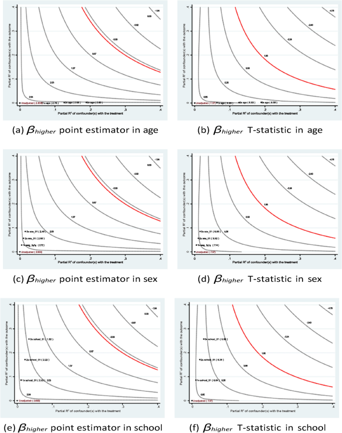
Sensitivity analysis of higher in Eq. (3) of case #2 in Portuguese.
This finding offers an additional perspective on the positive impact of government policies aimed at enhancing access to higher education. For instance, in 2024, the Chinese government outlined a set of refined financial aid policies to both reward outstanding students and support those from economically disadvantaged backgrounds. The number of National Scholarship recipients for both undergraduate and graduate students has doubled, accompanied by an increase in scholarship amounts. Such policies are likely to motivate high school students, particularly those facing financial hardship, to work harder, thereby contributing to improved educational outcomes at the K-12 level.
Case # 3. Class absences
The other explanatory variable that is highlighted three times by machine learning algorithms in the first stage is the number of class absences. In this section, this work studies the causal effect of absence on academic performance. While it might be apparent that more absences would drive down course grades, the goal of this case study is to complement the first two stages of the pipeline to demonstrate the procedure of the model-driven causal inference.
The following linear regression is estimated:
$$Grade{3}_{i} = \beta_{0} + \beta_{{1}} Absences_{i} + \gamma Controls_{i} + \varepsilon_{i} ,$$
(4)
where Absencesi is a numerical value ranging from 0 to 93 and the set of control variables is inherited from the results of post-double-LASSO.
In addition to the potential omitted variable bias induced by the unobserved student ability, another major empirical threat to Eq. (3) above is reverse causality, where absences could be a result of unsatisfactory course grades. Therefore, the study instruments Absencei by Goouti, which records the frequency of social activities. The IV relevance assumption is met here since interest in social activities might motivate the student to skip classes. The IV exclusion restriction is satisfied, as Goouti is only selected once in the first-stage results. The variable is still deemed relevant by LASSO regression in stage 1. However, Goouti is the most appropriate IV for Absencesi given data availability.
Tables 10 and 11 exhibit regression coefficients under different setups of the model. To avoid potential bias in the estimates induced by unusual and large values of Absencesi, this research also shows the estimated coefficients of the truncated sample, where only students who missed fewer than 22 or 30 classes are used in estimation. The p values for the underidentification test, which are 0.0571 (G3/G2/G1 <22) and 0.0833 (G3/G2/G1 <30), in Stata (i.e., the test of whether the matrices of all endogenous regressors and IVs are of full column rank). In almost all settings, the test is passed at the 10% confidence level.
The use of IV allows us to interpret the result as causal. Specifically, it is shown that each additional absence from class leads to a decline of 0.6 to 0.76 points in Portuguese. However, the impact of absences on course grades in Math is not significant. This might be due to the intrinsic difference between learning linguistics and science, where the former relies more heavily upon class participation, while the latter could be largely self-studied.
This finding aligns with existing research (e.g., see45 and more recently46) and provides statistical support for the widespread policy of recording attendance across various levels of education worldwide.
link


![Student Loan Debt Statistics [2026]: Average + Total Debt Student Loan Debt Statistics [2026]: Average + Total Debt](https://educationdata.org/wp-content/uploads/2025/03/page-1-3.png)


