A novel seven-tier framework for the classification of MEFV missense variants using adaptive and rigid classifiers

Exploratory data analysis

First, to evaluate feature relationships, we assessed 42 scores using Spearman correlations within three categories—LB, VOUS, and LP (Fig. 3A–C). Second, we applied principal component analysis (PCA) across 42 in silico tools, revealing that two principal components can explain 84% of the variance (Fig. 3D). Next, we selected the performance metric for LB and LP variant prediction. We identified the dataset as unbalanced and selected the F1 score as the performance metric (Fig. 3E).

Feature selection steps in the application of machine learning algorithms. Subfigures (A), (B), and (C) display Spearman correlation heatmaps for the LB, VOUS, and LP variants, respectively. Subfigure (D) illustrates the results of principal component analysis (PCA) applied across 42 in silico tools, revealing that the accessible in silico tools can be explained with two or three components. PC1 explains 60% of the variance, PC2 explains 24%, and PC3 explains 4% of the variance, together they account for 88% of the total variance. The elbow plot analysis suggests that using two components is more appropriate than three, as the additional component provides minimal improvement in clustering performance. (E) This classification system was further utilized to assess the distribution of amino acid positions. (F) The method employed for feature selection is recursive feature elimination with cross-validation (RFECV), which identifies six in silico tools as the optimal feature set for precise variant classification. The results underscore the effectiveness of these tools in distinguishing between different variant categories. (G) Feature importance metrics based on RF algorithm. Revel displayed outperformed performance than other scores. Determination of optimum number of clusters according to the Elbow Method (H) and Silhouette Scores (I). According to elbow method and Silhouette scores 3 number of clusters showed best overall performance (J) 3-means clustering results: Revel(First cluster), Mutation Assesor, MetaLR (Second cluster), CADD, SIFT, Polyphen-2 (Third Cluster). (Hyperparameters: n_clusters=[2, 3, 4, 5], init=’k-means++’, n_init = 10, max_iter = 300, tol = 1e−4, distance_metric=’euclidean’, random_state = 42, verbose = 0, algorithm=’lloyd’). Subfigures (K), (L), and (M), present the Spearman correlation analysis between LP, LB, overall (LP + LB) conducted on the top six selected in silico tools. The performance of the classification models is evaluated via F1 metrics, with the corresponding F1 scores displayed in subfigure. According to the RFECV scores and PCA, three in silico tools represent the optimum number of features. (N) The classifier’s performance was evaluated using RFECV and obtained the highest results with three features.

Feature selection

Feature selection is usually divided into three categories, namely filter, embedded, and wrapper methods. In our analysis, we applied these three techniques using the appropriate approach depending on the nature of the data that was given to us. For the filter method, we ranked features according to their correlation coefficients. For the embedded method, we used feature importance measures computed from a random forest model. Lastly, for the wrapper method, we used Recursive Feature Elimination with Cross-Validation (RFECV).

Determining the optimal number of features for machine learning models

In the fourth step, we use RFECV to test how many features the model can achieve the highest level of success with. For this purpose, we used the random forest method, which is relatively more sensitive to outliers than linear methods are. For this purpose, we included 42 in silico tools in a model. We imputed all missing values using tree-based methods²⁹. We determined that the optimal feature was three or six in silico tools (Fig. 3F) (Table 3). We calculated feature importance metrics for six features using the Random Forest algorithm. Based on these metrics, we derived the REVEL, SIFT, PolyPhen-2, MetaLR, CADD, and Mutation Assessor scores (Fig. 3G). To evaluate whether these features could be utilized more effectively, we decided to perform k-means clustering analysis. We initially determined the ideal number of clusters for this purpose by calculating the Elbow Method (Fig. 3H) and Silhouette Scores (Fig. 3I). The analyses indicated that three clusters were optimal. The clustering analysis identified REVEL as a unique cluster, MetaLR, and Mutation Assessor in the second cluster, and CADD, SIFT, and PolyPhen-2 in the third cluster (Fig. 3J). Furthermore, we noted high correlations among features within identical clusters (The clustering evaluation metrics were as follows: Silhouette Score = 0.56, Davies-Bouldin Index = 0.44, and ANOVA (F = 24.07, p = 0.014). Welch t-test revealed the following results: Cluster 0 vs. Cluster 1 (t = − 3.30, p = 0.183), Cluster 0 versus Cluster 2 (t = − 12.49, p = 0.041), and Cluster 1 vs. Cluster 2 (t = − 2.72, p = 0.156), indicating significant differences only between Cluster 0 and Cluster 2).

It is therefore important to remove features that are highly correlated as they are more likely to cause overfitting as pointed out by prior studies^9,12,30,31. To this end, we conducted Spearman correlation analysis of all six features and found that some scores were highly correlated (r > 0.7)^17,30,32,33 (Fig. 3K–M). After the RFECV, RFE, clustering analysis and correlation analysis, we have decided to reduce model feature numbers to obtain more optimum results. For this purpose, we decided to perform an analysis in such a way that one algorithm is selected from each cluster. We then performed the RFECV analysis again using RF (Fig. 3N). The model obtained similar performance metrics using three features in a shorter amount of time compared to using six features. We detected a noticeable improvement of 0.057 s (Table 2).

Feature selection steps

REVEL demonstrated significantly higher feature importance compared to other scores. MetaLR also outperformed Mutation Assessor in terms of feature importance. The previously described method imputed 42 missing values from Mutation Assessor, whereas MetaLR had no missing data. Furthermore, we observed a strong correlation between MetaLR and Mutation Assessor. These findings led us to choose MetaLR as the second feature for our model. Although the decision between MetaLR and Mutation Assessor was straightforward, selecting the third score was more challenging. PolyPhen-2, despite having a lower impact compared to other features, exhibited an influence level significantly below that of the first two scores. However, while CADD showed relatively higher feature importance than SIFT, the inherent negative correlation model in SIFT’s algorithm provided a safeguard against overfitting. To address these complexities, we decided to test all six possible combinations of the four scores using machine learning models without any preprocessing.

We looked at different three-feature combinations in the random forest model, including REVEL + MetaLR + Mutation Assessor, REVEL + MetaLR + CADD, REVEL + MetaLR + PolyPhen-2, and REVEL + MetaLR + SIFT. We found that REVEL and MetaLR were the two most important features in all of them. However, since the third feature varied across models, we opted not to rely solely on a model specific to the random forest algorithm. To address this, we tested all three-feature models across six machine learning algorithms and selected the combination with the smallest differences in F1 metrics. For these six algorithms, we chose three boosting methods, two bagging methods, and one linear method. The inclusion of a linear method allowed us to evaluate whether the chosen combination performed similarly in linear models. This approach ultimately led us to select SIFT as the third feature (Table 4). Had we relied solely on the random forest algorithm, we would have selected CADD as the third score. Consequently, we would have missed the combination with SIFT, which demonstrated relatively better performance in linear models (Supplementary Table 1).

Feature engineering

We detected 412 known MEFV gene variants in total. First, we checked our variants to detect the distribution type. Following this procedure, we removed from the model the 15 of 20 (75%) variants that were already known¹ and determined them by ClinVar’s two-star reviewer status. The motivation for not removing all 23 identified two-star variants was to maintain equilibrium between the LB and LP variants. There were only 7 LB/B (30.44%) variants, but there were 16 LP/P (69.46%) variants ( We did this to set them aside for testing the prediction performance of the model. Overall, 397 variants remained. The data, from both LP and LB variants, did not show a normal distribution based on the results of the Shapiro-Wilk, Anderson-Darling, and Kolmogorov-Smirnov tests in all three in silico tools (p < 0.001). Therefore, we performed log-scaled transformation for all the scores (Fig. 4A–C). However, the distribution was not altered (Fig. 4D). In this case, we opted to use a multivariate outlier analysis method. However, before proceeding, we considered evaluating the impact of outliers on the model using SHAP values. Completely removing these outliers could have resulted in a significant loss, both biologically and statistically, especially for Revel and MetaLR (Fig. 4F–G). Upon examining the dataset, it became clear that outliers varied across different scores. Therefore, a method capable of assessing these outliers in a multivariate context was required. In the next step, we implement multivariate outlier detection methods. We conducted LOF analysis on the basis of the optimal values of the hyperparameters. While conducting the analysis, we ensured there was no contamination and optimized the hyperparameters to retain as much data as possible while removing extreme outliers (n_neighbors = 20, contamination = 0.1, metric=’minkowski’, leaf_size = 20, p = 5); outlier_mask = lof.fit_predict(X) != -1). We were aware that this process might lead to the loss of biologically significant variants during model training. Therefore, while applying the LOF analysis, we focused on three important aspects: (1) We tested the best combinations for LOF analysis by optimizing all neighborhood sizes and contamination levels through hyperparameter tuning and used outlier thresholds of -1, -2, and − 3. Another potential approach could have been to reweigh the outliers. We compared the results of applying, weighting, and not applying LOF and found that removing outliers produced the best combination for LOF (Table 5). As a result, we identified 5 extreme values and eliminated 23 outliers from the study. Overall, after performing local outlier factor analysis, we obtained 369 variants (Fig. 4E). The SHAP analysis revealed that MetaLR had the largest contribution to the model’s predictions (-0.33), influencing outputs in a negative direction. In contrast, Revel (0.06) and SIFT (0.03) contributed positively, albeit minimally (Fig. 4F–H). While SHAP values indicated MetaLR’s dominant influence, other feature importance analyses identified Revel as the most significant feature overall, contributing to approximately half of the model’s predictive power (Fig. 4I).

Feature Engineering Steps in the Application of Machine Learning Algorithms. Subfigures (A), (B), and (C) present the log-transformed distributions and Q‒Q plots of the REVEL, MetaLR, and SIFT scores, respectively. For each subfigure, the left panels depict the log-transformed distributions, whereas the right panels present the corresponding Q‒Q plots. Subfigure (D) shows the combined density plots for the selected in silico tools, where nonnormal distributions persist even after data transformation (E). The 3D scatter plot (E) provides a visual representation of the local outlier factor (LOF) analysis, identifying and highlighting the 28 outliers that were subsequently excluded from the study. Subfigure (F) presents a heatmap of SHAP values, illustrating the impact of each feature on model predictions across instances. The dot plot in (G) further elaborates on the feature impacts, whereas subfigure (H) offers a summary plot of SHAP values, demonstrating the combined influence of the top features within the triple in silico tool model. Notably, MetaLR has a substantial negative effect on the model’s output. Finally, in subfigure (I), the feature importance metrics reveal that REVEL is the most significant contributor, accounting for approximately half of the model’s predictive power.

Model building and validation

After these steps, we implement training, validation, and test datasets into an ensemble classification dataset. We obtained better 10-fold cross-validation results. We analyzed known variants in two datasets: the training dataset (n = 291) and the test dataset (n = 78) after the outlier detection step. After implementing the machine learning algorithm, we conducted hyperparameter tuning for our accurate machine learning classifier algorithms (Supplementary Table 2). After hyperparameter tuning, the XGBoost and ExTC algorithms both displayed nearly perfect performance (Supplementary Table 3). Accordingly, all three voting classifiers, ExTC and AdaBoost, performed with perfect classification accuracy. However, we detected XGBoost and RF with relatively low precision scores. We tested the model’s prediction accuracy on 15 previously known ClinVar variants. The model correctly classified all 15 known variants via the hard, soft, and hybrid voting classifier methods (100%) (Fig. 5). Supplementary Tables 4 and 5 display the performance metrics of the remaining supervised machine learning models on both raw and preprocessed data, respectively. Among them, the LGBM classifier, label propagation, and bagging classifier indicated superior performance compared to other models. Surprisingly, the LGBM model demonstrated better performance metrics compared to XGBoost. In this context, we might be using the LGBM classifier instead of XGBoost. However, the study design phase is unlikely to predict such an outcome, as XGBoost typically favors relatively smaller datasets, while LGBM typically handles larger datasets. In this regard, the selection of XGBoost for the current dataset remains a more reasonable choice.

Evaluation metrics and performance comparison of different machine learning models employed in the classification of MEFV gene variants. Every subfigure provides detailed information about different aspects of the model’s training, validation, and performance. Visual representation of the learning curves, discrimination thresholds for each model, precision‒recall tradeoff, and class prediction error of all four algorithms (RF, ExTC, AdaBoost, and XGBoost). Accuracy metrics of all four algorithms with 5-fold cross-validation and hold-out methods: RF: 0.9788 ± 0.0158, ExTC: 0.9835 ± 0.0335, XGBoost: 0.9882 ± 0.0295, AdaBoost: 0.9671 ± 0.0815. Best hyperparameters for RF {max_depth’: 20, ‘min_samples_leaf’: 1, ‘min_samples_split’: 5, ‘n_estimators’: 200}, Best hyperparameters for ExTC: {‘max_depth’: 20, ‘min_samples_ leaf’: 1, ‘min_samples_split’: 2, ‘n_estimators’: 100}, Best hyperparameters for XGBoost: {‘learning_rate’: 0.1, ‘max_depth’: 5, ‘n_estimators’: 100}, Best hyperparameters for AdaBoost: {‘learning_rate’: 1, ‘n_estimators’: 200}

Model prediction of variations in unknown significance variants

The adaptive classifier classified 95.39% of VOUS variants, including both first-tier and second-tier categories, as LP or LB categories. Of these, 4.61% were classified as VOUS0 which means that they were not assigned to any category. On the other hand, the rigid classisfier was able to classify 64.78% of the second-tier VOUS variants. Still, 35.22% of the VOUS variants couldn’t be assigned to any of the categories in rigid classification system.

Clustering analysis

Method selection

We used distance-based methods for clustering analysis. Specifically, we employed agglomerative hierarchical clustering among distance-based methods and k-means among partitional clustering³⁴. We chose hierarchical clustering because we wanted to determine the optimal number of clusters in the 7-tier classification, which is based on an ordinal classification system, and to identify distances between clusters. For this analysis, we used Ward’s distance. We opted for a hard (strict) clustering algorithm instead of a fuzzy clustering algorithm to reduce the uncertainties that can arise with fuzzy clustering and to ensure that each variant belongs to exactly one cluster.

Application

We applied clustering analyses to three groups of data:

1. 1.

   A dataset obtained by simplifying the ClinVar dataset and producing a 7-tier classification.

2. 2.

   A dataset in which 1st-tier variants are considered LB (likely benign) and LP (likely pathogenic) as indicated by the Rigid Classifier.

3. 3.

   A dataset in which both 1st-tier and 2nd-tier VOUS (variants of uncertain significance) are considered LB and LP, as specified by the Adaptive Classifier.

Motivation

Our goal in the first phase was to determine into which groups the 7-tier classifier distributes the data and to assess the extent to which it reduces uncertainty. In the second phase, we aimed to identify which classifier—rigid or adaptive—could provide better separation metrics when VOUS variants are subdivided. We sought to adapt the results of the 7-tier classifier to both rigid and adaptive classifiers to see which models show alignment with clustering analyses performed without labels (Fig. 6)^{28,35,36,37,38}.

Flowchart of clustering methods.

With this objective, we first set out to determine the optimal number of clusters for both the k-means and hierarchical clustering algorithms. Accordingly, out of the 22 methods used for hierarchical clustering, 9 (41%) identified 3 as the optimal number of clusters, and out of the 29 methods used for k-means, 11 (39%) also identified 3 as the optimal number of clusters^39,40,41 (Supplementary Tables 6 and 7, respectively). In the next step, we performed both k-means and hierarchical clustering and compared the distributions in these clusters. These analyses are presented in Figs. 7 and 8, respectively.

K-means Clustering Results (A) Overall distribution of the dataset obtained via the 3-means (K-means) clustering method; (B) distribution of the 412 known variants. (C,D) In the K-means analysis, Cluster 3 is designated as the LP variant–dominant cluster and Cluster 2 as the LB variant–dominant cluster, while Cluster 1 lacks a distinct group-specific distribution pattern and is thus classified as the VOUS cluster irrespective of variant counts or percentages. (E–H) Similarly, the hierarchical clustering approach applied to the same dataset produced comparable distribution patterns. In a subsequent analysis, variant distributions were further examined using both rigid and adaptive classifiers; notably, the application of the adaptive classifier enhanced intra-cluster homogeneity and reduced inter-cluster heterogeneity.

Hierarchical clustering Results. (A) Overall distribution obtained using hierarchical clustering analysis (n = 3). (B) Distribution of the 412 known variants. (C,D) In the analysis, Cluster 1 was found to be dominated by LP variants, whereas Cluster 2 primarily comprised LB variants. Cluster 3 did not exhibit any distinct group-specific distribution in terms of either the number or proportion of variants and is thus defined as the VOUS cluster. (E–H) In a subsequent evaluation, variant distributions were analyzed using both rigid and adaptive classifier approaches; the adaptive classifier approach was observed to enhance intra-cluster homogeneity while diminishing inter-cluster heterogeneity.

Interpretation of results

K-means clustering

According to the results of the 7-tier classification, the third cluster mainly contained LP, VOUS++, and VOUS + variants (95.6% of third cluster). In this classification, only a small number of LB variants were identified in the third cluster, making it the cluster with the fewest LB variants (2.3% of third cluster); moreover, it contained only four VOUS–, and VOUS- variants (0.5% in third cluster). Meanwhile, the second cluster included LB, VOUS–, and VOUS–– variants (89.3% of third cluster). It contained only a limited number of LP variants (3.7% of third cluster). Hence, the first two clusters showed a clear separation in terms of classification. Therefore, we labeled the third cluster as the LP variant cluster and the second cluster as the LB variant cluster. Another important reason for this labeling was that all two-star LP/P variants from ClinVar were located in the first cluster, whereas the remaining LB/B variants were located in the second cluster (Fig. 7C,D).

However, the first cluster did not exhibit a distinct pattern based on variant types. Altogether, the second and third clusters contained a substantial portion of the total variants. If we assume that 35 variants (2.8% off all variants) in the third cluster (LP variant cluster) and 45 variants (4.3% of all variants) in the second cluster (LB variant cluster) were incorrectly assigned, then 1796 variants (a 29.35% out of all variants) could be considered properly clustered compatible with group names. By comparison, the simplified Clinvar dataset which we prepared for supervised learning (7-tier classification dataset) classifies a much smaller fraction of all variants (assumed 412 variants, confirmed 23 variants). Therefore, the k-means approach increased the number of assumed “known” variants by 412%.

Furthermore, when the known LB and LP variants (412 variants) were clustered into three groups, none of the clusters showed a statistically significant distribution (p > 0.05). In contrast, the 7-tier classification system enabled a more distinct clustering-based separation of LB and LP variants. After establishing that this separation occurs in such a manner, the next step was to determine the cutoff point for VOUS variants in the 7-tier classifier. For this, we used both rigid and adaptive classifiers(Fig. 7E–H). Under the adaptive classifier, the third cluster in the k-means analysis contained a high percentage (e.g., ~ 95.6%) of LP variants, whereas the second cluster contained a similarly high percentage (e.g., ~ 89.3%) of LB variants (Fig. 7G,H). Thus, both clusters achieved statistically significant separation (p < 0.001 for each). In the third cluster, the significant difference was driven by LP variants; in the second cluster, by LB variants. The rigid classifier, similar to the adaptive classifier, also significantly separated the second and third clusters (p < 0.001 for both).

Hierarchical clustering

According to the results of the 7-tier classification, the first cluster mainly contained LP, VOUS++, and VOUS + variants. In this classification, only 19 LB variants were identified, representing the cluster with the fewest LB variants; additionally, this cluster contained no VOUS– – or VOUS– variants. Meanwhile, the second cluster mainly contained LB, VOUS–, and VOUS–– variants. This cluster included only 29 LP variants and did not include any VOUS + or VOUS + + variants. Hence, the first two clusters showed a clear separation in terms of classification (Fig. 8C,D). Therefore, we labeled the first cluster as the LP variant cluster and the second cluster as the LB variant cluster. Another important reason for this decision was that all 16 LP/P variants with two-star ratings in ClinVar were located in the first cluster, while the other 7 LB/B variants were located in the second cluster.

However, the third cluster did not exhibit a distinct pattern based on variant types. Altogether, the first and second clusters contained 1,079 variants. If we assume that the 19 LB variants in the first cluster (LP variant cluster) and the 29 LP variants in the second cluster (LB variant cluster) were incorrectly assigned, then a total of 1,041 variants (17.59% of all variants) could be considered properly clustered. In contrast, the simplified ClinVar dataset—comprising 412 variants in its most reduced form—classifies only 6.96% of all variants. Therefore, our approach increased the number of assumed “known” variants by 152.73%. Furthermore, when these 412 known variants (LB and LP) were clustered into three groups, none of the clusters showed a clear distribution (p > 0.05). In contrast, the 7-tier classification system enabled a more distinct clustering-based separation of LB and LP.

After identifying that this separation occurs in this manner, the next step was to determine the cutoff point for VOUS variants in the 7-tier classifier. For this, we used rigid and adaptive classifiers. In the hierarchical clustering analysis under the adaptive classifier, 95% of the variants in the first cluster were in the LP category, and 93% of the variants in the second cluster were LB. Thus, both clusters achieved statistically significant separation (p < 0.001 for each). In the first cluster, the significant difference was driven by LP variants; in the second cluster, by LB variants. The rigid classifier, similar to the adaptive classifier, was able to significantly separate the variants in the first and second clusters (p < 0.001 for both) (Fig. 8E–H). In the first cluster, the significant difference arose from LP variants, whereas in the second cluster, it arose from non-LP variants (p < 0.001 for both).

External validation steps results

According to the results of both k-means and hierarchical clustering, the adaptive classifier yielded higher NMI and ARI scores compared to both the rigid classifier and the original three-tier classification (LB, VOUS, LP) (p < 0.05 for both NMI and ARI scores). The scores for the original classification and the rigid classification, however, were similar to each other (P > 0.05) (Fig. 9A–D). For this reason, we planned to make the final classification by partitioning the groups in accordance with the adaptive classifier.

Comparison of External Validation Metrics. (A) External Validation metrics comparison among Rigid, Adaptive, and Seven-Tier Classifiers. (B–D) An ANOVA/Kruskal–Wallis’s test on the [ARI/NMI/Purity] distributions revealed a significant overall effect (p < 0.05). Post-hoc comparisons (Tukey/Dunn) indicated that the Adaptive Classifier’s mean score differs significantly from both the Original and Rigid classifiers (p < 0.05), whereas no significant difference was observed between the Original and Rigid classifiers.

Final classification

The execution of the final categorization is illustrated in Fig. 10A. Prior to the establishment of the 7-tier classification system, 6.9% of the total variations were categorized as “known.” Following the refinement of the dataset and the implementation of a novel classification and clustering methodology, that proportion increased to 29.4%. This leap signifies a rise of 22.5% points, or almost a 4.3-fold relative increase. The revised method or dataset more precisely identifies known variants, significantly enhancing their recognition within the total collection (Fig. 10B–D).

Final Classification Scheme, Results and Comparative Datasets. (A) Flowchart outlining the final classification results. Panels (B) and (C) present the ClinVar classification dataset, derived from Ensembl and employed for a simplified analysis; this comparison incorporates the raw dataset used for supervised algorithm training, wherein the set of 412 known variants is presumed to represent 6.9% of the total dataset. Panels (D) and (E) include the 7-tier classification dataset, accounting for a total of 1744 variants (29.4% of the entire dataset).

Implementation of biological processed systems

In the subsequent stage, a potential three-stage clustering approach was implemented to evaluate the distribution of VOUS, LB, and LP variants across the identified clusters. This approach was applied to the 7-tier classification method, amino acid polarity status, and protein domains. For each parameter, the most suitable separation thresholds were determined (Supplementary Figs. 1–3).

Hotspot region prediction

Since the VOUS + + and VOUS + + predictions contain prediction patterns that are relatively closer to LP, when we cluster the regions containing these two predictions according to the other three VOUS subtypes (VOUS0, VOUS-, VOUS–), we alternatively obtained three significant regions (Fig. 11A). We did not include the LP and LB variants in this cluster, as this may introduce bias into the training dataset. Therefore, we only used the prediction dataset.

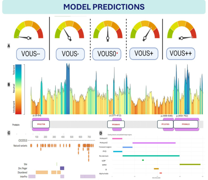
Model Predictions on Existing Domains (A) Seven-Tier Classification System, Ordinary 5-tier VOUS classification system (B) Protein tolerance landscape and domain mapping of pyrin protein (PF02758: PAAD/DAPIN/Pyrin domain, PF00643: B-box zinc finger, PF13765: SPRY-associated domain, PF00622: SPRY domain, GENCODE: ENST00000219596.1, RefSeq: NM_000243.2, UniProt: O15553) (C) The distributions of pyrin protein regions can be predicted via SWISS-MODEL. (Protein structure predictions for O15553 were obtained from SWISS-MODEL (https://swissmodel.expasy.org/repository/uniprot/O15553) under the Creative Commons Attribution 4.0 (CC BY 4.0) license. For further details, see Waterhouse et al., Nucleic Acids Res. 46, W296–W303 (2018). DOI: (D) Existing domains, alternative predicted hotspot and tolerant regions. Two hotspot and one tolerant region predicted on the basis of VOUS variants. We did not include the LP and LB variants in this cluster, as their inclusion could introduce bias. The MEFV prediction app provides detailed information.

MetaDome is a web server that depicts genetic tolerance profiles across genes and specific protein domains by aggregating population variation and pathogenic mutations onto meta-domains at the level of amino acids⁴², and is widely used by genetic studies for structural and functional in silico analysis^43,44. The MEFV gene encodes the three-dimensional structure of pyrin (Supplementary Fig. 4), which consists of modular domains such as an N-terminal pyrin domain (PYD) for inflammasome assembly, coiled-coil and B-box domains for structural integrity, and a C-terminal B30.2 (PRY-SPRY) domain involved in molecular recognition and autoinflammatory regulation¹. According to the metadome browser, many MEFV gene hotspot regions most likely do not contain domains except SPRY-associated domains and pyrin domains (Fig. 11B). That is compatible with “evolutionary conservation does not mean includes hotspot region” and many examples are available⁴⁵. Particulary, many hotspot regions in MEFV gene does not contain domains. Many intolerant regions detected outside of the domain regions^9,46. For example, the region between amino acids 451 and 600 is considered a hotspot region, despite not containing any domains. In our model, this region is designated as “hotspot2.” Additionally, regions of significant genetic intolerance in the MEFV gene begin prior to position 190 and extend to include the hotspot2 region, continuing until position 600. The SPRY domain, which is the largest domain in the MEFV gene²⁰, is associated with 12 P/LP variants and is responsible for a substantial portion of MEFV-related clinical manifestation according to Clinvar (3/12/2024). However, aside from the mutations identified in this domain, no significant alterations that disrupt protein structure have been reported¹ and does not explain the exact relationship with FMF disease⁴⁷. In fact, the most tolerable regions of the protein are also found within this domain. Consistent with this observation, our model neither classified this domain as a hotspot nor as a tolerable region.

However, the model predicted the region between amino acids 105 and 185 as a tolerable area, albeit starting at position 90. This caused the model to overlook the intolerant region between amino acids 90 and 112, highlighting a limitation of the current design. A notable success of the model is its precise alignment of hotspot 1 with the pyrin domain. The model also correctly predicted potential regions outside of domains, excluding SPRY, SPRY-associated, and pyrin domains, which shows a high level of accuracy. Nevertheless, the model failed to predict the zinc-finger domain located between amino acids 371 and 412. Despite this, it identified potential domains in three out of the four major domains, which is commendable.

Notably, the model’s prediction of the 451–600 region as a hotspot while distinguishing it from SPRY and SPRY-associated domains is a remarkable achievement. Additionally, the model’s ability to precisely predict the pyrin domain as a hotspot, despite missing certain other hotspot regions, underscores its potential. While the model demonstrates a reasonable predictive performance for hotspot and non-domain regions, there is substantial room for improvement. As a prototype, it is valuable in its current form but remains constrained by the limitations inherent to in silico tools and their reliance on ClinVar-reported variants. These predictions are not based on experimental or clinical study data. Therefore, the limitations of the model should be interpreted within the context of study design and resource constraints. In conclusion, our model suggests several alternative domain regions in addition to those predicted by many other protein prediction tools (Fig. 11C–D)^42,48.