
A deep learning based intrusion detection system for CAN vehicle based on combination of triple attention mechanism and GGO algorithm

In the present part, the approaches utilized in the suggested intrusion recognition and Controller Area Network are presented. Initially, the convolutional neural network used in this work has been introduced, then the adversarial generator network, and the controller area network have been evaluated.
Triple-attention mechanism
The mechanism of attention is famous for probability weight distribution. It calculates the attributes at diverse times, hence the features that have more data are able to learn better weighting coefficients. Therefore, it can enhance the high-dimensional hidden layer attributes’ quality. The mechanism of triple attention has been utilized as a weighted sum of top-p local attributes in a dynamic manner to obtain a local attribute \(d_j\) (Eq. 1). In other words, \(H_j\) equals \(H_k ,H_k ,H_j , \ldots ,H_j\).
$$d_j = \mathop \sum \limits_j^j b_k H_k$$
(1)
where the features’ weight coefficient has been represented by \(k_k\) within the sequence of input. By taking into account the functions of attention, the score of relevance \(f_j\) are mathematically represented in Eq. (2):
$$f_k = x_j^{U} {\text{tanh}}\left( {X_{f} H_{u – 1} + V_{f} H_{jk} + a_{f} } \right)$$
(2)
where the attribute points of \(k\) has been demonstrated via \(m\), the pixel \(k\)’s hidden state data has been illustrated via \(H_{k}\) by vectors of feature. Ultimately, the summary function of hidden state \(b_{jk}\) and \(h_{k}\) has been utilized for creating vector of context \(d_{j}\). Also, the shared variables have been depicted through \(X_{f}\), \(x_{m}^{U}\), \(a_{f}\), and \(V_{f}\). After that, the attention weight \(b_{jk}\) has been calculated in Eq. (3):
$$b_{jk} = \frac{{{\text{exp}}\left( {f_{jk} } \right)}}{{\mathop \sum \nolimits_{l = 1}^{p} {\text{exp}}\left( {f_{jl} } \right)}}$$
(3)
In the suggested study, a triple-attentional mechanism includes 3 diverse modules of attention, including max-pooling attention, average pooling attention, and traditional attention mechanisms. The initial attention mechanism preserves half of features with more weight. In the following, the max-pooling attention mechanism emphasizes the local attributes with more weight. In the end, the average pooling function has been used to maintain local attributes. These modules of attention have been computed subsequently:
$$O = \mathop \sum \limits_{k = 1}^{p} \frac{{{\text{exp}}\left( {f_{jk} } \right)}}{{\mathop \sum \nolimits_{l = 1}^{p} {\text{exp}}\left( {f_{jl} } \right)}}$$
(4)
$$h = AVG.POOLING\left[ {\mathop \sum \limits_{k = 1}^{p} \frac{{{\text{exp}}\left( {f_{jk} } \right)}}{{\mathop \sum \nolimits_{l = 1}^{p} {\text{exp}}\left( {f_{jl} } \right)}}H_{jk} } \right]$$
(5)
$$n = MAX.POOLING\left[ {\mathop \sum \limits_{k = 1}^{p} \frac{{{\text{exp}}\left( {f_{jk} } \right)}}{{\mathop \sum \nolimits_{l = 1}^{p} {\text{exp}}\left( {f_{jl} } \right)}}H_{jk} } \right]$$
(6)
where the outcome of the mechanism attribute of traditional attention has been represented via \(O\), the outcome of the mechanism feature of the average pooled attention has been displayed via \(n\), and the outcomes of the mechanism feature of the maximum pooled attention has been demonstrated via \(h\).
Additionally, several weights have been allocated through triple-attention mechanism to the real intrusion detection, which can distinguish all the features. The integrated output formula of the current mechanism has been computed in Eq. (7):
$$G_{{\left( {O,h,n} \right)}} = Concatenate\left( {O \oplus h \oplus m} \right)$$
(7)
When the distribution and computation processes have been conducted by the mechanism of attention, three diverse features with novel weights are generated via the weights optimizer. The integrated result of triple-attention attributes has been resembled by \(G_{{\left( {O,h,n} \right)}}\). the procedure of the feature fusion optimizer has been displayed via \(\oplus\). The fusion features’ output provides a denser residual network that have more depth attributes by integrating multiple-attention structures.
Dense residual network
The dense residual network has been created for combining deep attributes. The distinction between the residual network and the conventional convolutional network is that the former one can offer a skip residual procedure. the current procedure can minimize the characteristic variables; moreover, it omits the vanishing gradient and degradation initiated through deep features. The residual network has been calculated in Eq. (8):
$$Z = X_{j\gamma } \left( {X_{j – 1} Y_{j – 1} } \right) + Y$$
(8)
where the layer’s output has been represented through \(Z\), and the activation function of ReLU has been resembled via \(\gamma\). The weight matrix and the present layer input have been demonstrated through \(X\) and \(Y\). Considering the feature fusions, the previous data offered by the dense network presents a huge amount of previous feature to mine deep attributes, hence maintaining massive deep attributes. The double dense fusion policy has been resembled in the current study because it performs a feature fusion procedure using initial features and deep residual. To accomplish additional deep features, the initial and deep residual features have been thoroughly utilized by the policy of double dense fusion. The deep residual and initial features have been computed in Eqs. (9) and (10)
$$Y_{0} = I_{\partial } \left( {Y_{\partial – 1} } \right) + Y_{\partial – 1}$$
(9)
$$Y_{Z} = I_{\partial } \left( {Y_{\partial – 1} } \right) + Z_{\partial – 1}$$
(10)
where the intensive operation of initial attributes has been demonstrated through \(Y_{0}\), the policy of feature fusion has been depicted through \(I_{\partial }\), the output features’ intensive operation in the residual network has been demonstrated by \(Y_{Z}\). Rapid Tri-Net can mine the feature deeper and the fusion of the high-dimensional data. Moreover, it can solve the problems related to the gradient disappearance and explosion in deep network.
Capsule network
The capsule network has been introduced to maintain the situation of objects and their characteristics in data. It generates a vector output of akin size with different routings. These vector routings represent the parameters of the data. Conventional neural networks (CNNs) employ scalar input activation functions, such as tangent, sigmoid, and ReLU. In contrast, the capsule network makes use of a vector-based activation function known as squashing, which is illustrated in the subsequent equation.
$$w_{k} = \frac{{\left\| {T_{k} } \right\|^{2} }}{{1 + \left\| {T_{k} } \right\|^{2} }}\frac{{T_{k} }}{{\left\| {T_{k} } \right\|}}$$
(11)
where the input and output vectors of the capsule \(k\) have been, in turn, represented through \(T_{k}\) and \(w_{k}\). Once there exists an entity within the data, \(w_{k}\) decreases a long vector near 1. Whereas, it there exists no entity within the data, \(w_{k}\) decreases a short vector near 0. The capsule \(T_{k}\)’s entire input value has been calculated by the weighted total amount of the vector (\(V_{k|j}\)) within the capsule, which has been located in the lower layers, and it excludes the capsule network’s initial layer (Eqs. 12 and 13). The vector has been computed through multiplication of capsule layer within the lower layers by the weighted matrix (\(V_{k|j}\)) and its findings \(P_{j}\).
$$T_{k} = \mathop \sum \limits_{j} c_{jk} v_{k|j}$$
(12)
$$v_{k|j} = X_{jk} P_{j}$$
(13)
where the coefficient calculated by the dynamic routing procedure has been represented through \(c_{jk}\), which has been calculated in the following way:
$$c_{jk} = \frac{{{\text{exp}}\left( {b_{jk} } \right)}}{{\mathop \sum \nolimits_{l} {\text{exp}}\left( {b_{jl} } \right)}}$$
(14)
where the log probability has been displayed through \(b_{jk}\). The softmax is capable of determining the total amount of correlation coefficients between the log probability and the top layer’s capsule, as well as \(j{\text{th}}\) capsule. The loss of margin has been demonstrated within the capsule network for realizing if a specific category’s entities are accessible. This has been computed subsequently:
$$M_{l} = U_{l} Max\left( {0, n^{ + } – \left\| {w_{l} } \right\|} \right)^{2} + \kappa \left( {1 – U_{l} } \right)Max\left( {0, \left\| {w_{l} } \right\| – n^{ – } } \right)^{2}$$
(15)
The value of \({U}_{l}\) has been regarded as 1 once the category \(l\) exists. \({n}^{+} = 0.9\) and \({n}^{-} = 0.1\) have, in turn, represented hyper-parameters and down-weighting of the loss. The length of vector calculated within the capsule network demonstrates the probability that it might be in the data portion, while the direction vector includes the data of variables, such as texture, color, size, position, and so on.
In addition, the capsule network includes 3 fully connected layers, 1 digit layer, 1 primary layer, and 1 convolutional layer. The convolutional layer consists of 256 kernels with sizes of \(9 \times 9\), and it can transform pixel’s densities to local attributes with size of \(20 \times 20\) to be utilized like inputs within the initial capsule. The primary capsules’ subsequent layer consisted of 36 capsules, which utilized convolutional kernels with the size of \(9 \times 9 \times 9 \times 256\). These two-layer utilized ReLU activation function. Digital caps’ ultimate layers within 16D vectors consisted of instantiation variable required for reform.
In this study, we used a metaheuristic-based methodology for optimizing this network for providing optimal results in the system.
Novel Greylag Goose Optimization algorithm
The gooseneck’s most significant feature is the breeding manner during sperm forming and the way the wind and wave action influence the breeding. Thus, an algorithm was designed in order to imitate such features in a mathematical way. Subsequently, the mentioned model’s design has been displayed.
$$\left( {X + l} \right)_{i + 1} = { }\left( {X + l} \right)_{i} + WD_{i} + T_{dim} + S\left( {\left( {X + l} \right)_{i} ,(SP_{water} )_{j} } \right) + HS.{ }\left( {X + l} \right)_{i}$$
(16)
where the goose barnacle’s situation in \(i_{th}\) iteration has been demonstrated by \(\left( {X + l} \right)\), the wind’s orientation within \(i_{th}\) iteration has been displayed via \(WD\), \(T_{dim}\) has been considered the goal dimension for going through the best solution or the aim, \(S\left( {\left( {X + l} \right)_{i} ,(Sp_{water} )_{j} } \right)\), the logarithmic spiral amid the \(j_{th}\) sperm region inside water has been represented via \(S\), \(i_{th} \left( {X + l} \right)_{i}\) and \(Sp_{water}\), and the significant height of wave has been illustrated by \(Hs\). The comprehensive clarification of the model’s all mathematical stages is explained below.
Initialization
Within GBO algorithm, the gooseneck barnacles are the individual solution, and the goosenecks’ location are the problem space variables. The gooseneck is capable of traveling any dimensional space through spreading their penis, which may be seven or eight times larger than their body27. Actually, GBO is a population-based algorithm. So, for initialization, the individual solution \(X\) has been considered the gooseneck barnacles’ population, which is a kind of stalked barnacle and is demonstrated in the following:
$$X = \left[ {\begin{array}{*{20}c} {\begin{array}{*{20}c} {\left( {X + l} \right)_{1,1} } & {\left( {X + l} \right)_{1,2} \ldots } & {\left( {X + l} \right)_{1,d} } \\ \end{array} } \\ {\begin{array}{*{20}c} \vdots & \vdots & \vdots \\ \end{array} } \\ {\begin{array}{*{20}c} {\begin{array}{*{20}c} \vdots & \vdots & \vdots \\ \end{array} } \\ {\begin{array}{*{20}c} {\left( {X + l} \right)_{n,1} } & {\left( {X + l} \right)_{n,2} \ldots } & {\left( {X + l} \right)_{n,d} } \\ \end{array} } \\ \end{array} } \\ \end{array} } \right]$$
(17)
here, the entire populations have been displayed by \(n\), and the dimension as \(X\) or variables’ amount has been specified by \(d\). As the goosenecks have an eatable construction, all of them has different sizes, which have been displayed by \(l.\) that would be chosen in a random way. There would be a consistent area inside the water for all of the animals that has sperm in order to breed. Actually, this is an important factor in the suggested algorithm called as ‘sperm_region’ that its matrix is similar to \(X\):
$${\text{Sperm}}\_{\text{Region}} = \left[ {\begin{array}{*{20}c} {\begin{array}{*{20}c} {\left( {sr} \right)_{1,1} } & {\left( {sr} \right)_{1,2} \ldots } & {\left( {sr} \right)_{1,d} } \\ \end{array} } \\ {\begin{array}{*{20}c} \vdots & \vdots & \vdots \\ \end{array} } \\ {\begin{array}{*{20}c} {\begin{array}{*{20}c} \vdots & \vdots & \vdots \\ \end{array} } \\ {\begin{array}{*{20}c} {\left( {sr} \right)_{n,1} } & {\left( {sr} \right)_{n,2} \ldots } & {\left( {sr} \right)_{n,d} } \\ \end{array} } \\ \end{array} } \\ \end{array} } \right]$$
(18)
here, \(n\) has been the gooseneck’s amount, and \(d\) has been the dimension as \(X\) or variables’ quantity. While the two of gooseneck barnacles’ situation and regions of sperm are probable responses, the manner that the issue’s domain controls them in every iteration would differ. Actual search agents, such as the ones existing in the gooseneck barnacles’ penis, direct the solution space, although the area of sperm inside the water signifies the optimum reproducing place.
Because of breeding, the area of sperm might be supposed as the innovative gooseneck within the solution space. Therefore, the goosenecks discover the innovative location and improve it in the case that they discover a finer substitute. The present method guarantees that the optimum choice for a gooseneck would be obtainable all the time. Research show that Gooseneck barnacles are originated in the higher and middle intertidal areas.
The height of significant wave has been noticeably under 0.8 to 1.5–3 m beyond mean low water has been the supremacy for barnacles. Commonly, height of significant wave has been computed through the present equation \(Hs = 4\sqrt {H \wedge 2T}\), but, in the current form of GBO, the \(Hs\) would be computed via the subsequent formula. Actually, the barnacles’ tolerance in their cycle of life have been considered.
$$Hs = 1.5 – \left( {\frac{{Iteration \left( {1.5 – 0.2} \right)}}{maximum\;Iteration}} \right)$$
(19)
here, it is concluded that barnacle is capable of tolerating the intensity of wave ranging from 1.5 or 3.0 to 0.2 m. The Hs would be reducing within each iteration for exploring the wave intensity range for discovering the optimum reproducing area. Next, an adjoining logarithmic spiral area has been demonstrated for sperm casting.
$$S\left( {\left( {X + l} \right)_{i} (Sp_{water} )_{j} } \right) = D_{i} .e^{bt} .\cos \left( {2\pi t} \right) + (Sp_{water} )_{j}$$
(20)
here, the \(i_{th}\) barnacle’s distance for the area of \(j_{th}\) sperm for breeding has been represented via \(D_{i}\), the constant to define the logarithmic spiral’s shape has been represented via \(b\), and the stochastic amount in [1, -1] has been illustrated by \(t\). Distance has been computed this way: \(D_{i} = \left( {X + l} \right)_{i} , – (Sp_{water} )_{j}\). here, \(\left( {X + l} \right)_{i}\) shows the \(i_{th}\) barnacles, \((Sp_{water} )_{j}\) specifies the \(j_{th}\) sperm casting area, and \(D_{i}\) displays the \(i_{th}\) barnacles’ distance for the \(j_{th}\) sperm casting region.
Off-spring generation
The sperm-cast breeding manner has been considered to be the integration of some forms argued in the current study. For updating the position of innovative gooseneck barnacles within a solution space and mimicking the motion through novel progeny generation, a movement vector have been assumed, \(\Delta \left( {X + l} \right)_{i}\), which is displayed below:
$${\Delta }\left( {X + l} \right)_{i + 1} = WD_{i} + T_{dim} + Hs. {\Delta }\left( {X + l} \right)_{i}$$
(21)
$$\left( {X + l} \right)_{i + 1} = \left( {X + l} \right)_{i} + {\Delta }\left( {X + 1} \right)_{i + 1}$$
(22)
$$\left( {X + l} \right)_{i + 1} = \left( {X + l} \right)_{i} + Levy^{*} \left( {X + 1} \right)_{i}$$
(23)
The wind orientation has been displayed by \(WD_{i}\) that is resulted by the degree range [0 359] on the solution space radios, and lastly added with the target dimension \(T_{dim}\) to the finest solution. \(T_{dim}\) or dimension through target is considered the dimension’s value within the target, through considering wind orientation to the target all the time. here, Levy flight has been displayed:
$$Levy \left( N \right) = 0.01 \times \frac{{r_{1} \times \sigma }}{{|r_{2} |^{{\frac{1}{\beta }}} }}$$
(24)
\(\beta\) has been a constant that is set to 1.5, \(r1\) and \(r2\) have been stochastic amounts [0–1], and the formula is below:
$$\sigma = \left( {\frac{{\tau \left( {1 + \beta } \right) \times \sin (\frac{\pi \beta }{2})}}{{\tau \left( {\frac{1 + \beta }{2}} \right) \times \beta \times 2^{{\left( {\frac{\beta – 1}{2}} \right)}} }}} \right)$$
(25)
where \(\tau \left( y \right) = \left( {y – 1} \right)\).
The prior clarification displays that the present calculated model needs the gooseneck barnacle for moving through a goal breeding area within the logarithmic spiral area of sperm for sperm casting over some iterations. But, there are not any orientations in the real solution space since the situation of global optimal needs to be found. Therefore, within every optimization iteration, a reproducing aim should be selected. Within GBA, the gooseneck with the maximum objective value during optimization has been considered to be the objective that makes other goosenecks become nearer to the breeding zone, but, it aids GBA keep the most talented goal within the solution space throughout every replication.
In fact, the GBA starts the optimization procedure via producing a stochastic lake of individual solutions. After that, according to the Eq. (22), the search agents modify their locations through the objective as the wind orientation and significant wave movement. In order to mimic the actual situation there might be just single sperm area remained, based on the wave intensity of the wave and wind. If their location would be enhanced by means of Eq. (23). Lastly, iteratively improving the location has been accomplished till the last necessity has been met. Finally, the finest global approximation has been assumed, besides the quality and place of the finest objective. Although the earlier debates demonstrated the way the GBA algorithm has been effective at finding the greatest result in a solution space.
Novel version
Greylag goose optimization algorithm (GGO) is novel optimization algorithm that recently introduced. But it has some limitations in some problems. Between two data samples, this algorithm struggles to update the variable damages to the factors iteratively till the modal data equals the final achieved outcomes in the field structure. This reduces the exploration term of the algorithm and leads it to prematurely converge on it. The new exploitation term of the algorithm in the current work is framed based on the Cuckoo Search Algorithm (CS)28 and Gray Wolf Optimization (GWO)29. This improvement leads to the following general equations for updating:
$$\left( {X + l} \right)_{1} = \left( {X + l} \right)_{i} – A_{1} \times \left( {C_{1} \times \left( {X + l} \right)_{i}^{New} – \left( {X + l} \right)_{i} } \right)$$
(26)
$$\left( {X + l} \right)_{2} = \left( {X + l} \right)_{i} – A_{2} \times \left( {C_{2} \times \left( {X + l} \right)_{i}^{New} – \left( {X + l} \right)_{i} } \right)$$
(27)
$$\left( {X + l} \right)_{3} = \left( {X + l} \right)_{i} – A_{3} \times \left( {C_{3} \times \left( {X + l} \right)_{i}^{New} – \left( {X + l} \right)_{i} } \right)$$
(28)
$$\left( {X + l} \right)_{i + 1}^{New} = \frac{1}{3} \times \left[ {\left( {X + l} \right)_{1} + \left( {X + l} \right)_{2} + \left( {X + l} \right)_{3} } \right]$$
(29)
where \(\left( {X + l} \right)_{i}^{New}\) represents the new solution and \(A_{1}\), \(A_{2}\), \(A_{3}\) and \(C_{1}\), \(C_{2}\), \(C_{3}\) specify the generated from \(A_{i}\) and \(C_{i}\), where,
$$A = 2 \times a \times rnd_{1} – a$$
(30)
$$C = 2 \times rnd_{2}$$
(31)
where \(a\) determines the linearly decreasing, and \(rnd_{1}\) and \(rnd_{2}\) represent two random values in the range [0, 1].
This change is based on ideas from GWO and includes updating 50% of the algorithm. The other 50% of the updates during the process are inspired by the CS algorithm, as shown below:
$$\left( {X + l} \right)_{i + 1} = \left( {X + l} \right)_{i} + \alpha \otimes L\left( \lambda \right) \times \left( {\left( {X + l} \right)_{Best} – \left( {X + l} \right)_{i}^{New} } \right)$$
(32)
where \(\alpha\) and \(L\left( \lambda \right)\) specify the Lévy distributed random values.
Optimizing TAN based on NGGO algorithm
Metaheuristic algorithms are widely used to optimize the network in various architectures, including those based on the triple-attention module, dense residual network, and capsule network. What follows is a recommendation of how the objective function would be set, for the embedding space and a loss function that allows the model to minimize the preserving rules. Below is a more in depth look at how you could structure the objective function:
-
(A)
Loss Function of Attention Mechanism
The attention mechanism, such as the triple-attention mechanism, tends to dynamic-weight different features, which helps improve the quality of feature extraction. The attention mechanism optimization objective function can be represented as:
$$Loss_{attention} = – \mathop \sum \limits_{i = 1}^{N} \mathop \sum \limits_{j = 1}^{P} \left[ {y_{ij} \log \left( {d_{j} } \right) + \left( {1 – y_{ij} } \right)\log \left( {1 – d_{j} } \right)} \right]$$
(33)
where \(y_{ij}\) is the ground truth label of the \(i – th\) sample and \(j – th\) feature, \(d_{j} = output\) of the attention mechanism for the \(j – th\) feature, \(N\) is the number of samples, \(p\) signifies the number of features.
-
(B)
Loss Function for Dense Residual Network
The dense residual network is designed to reduce the vanishing gradient issue and enhance the ability to extract features. The goal of optimizing the dense residual network can be expressed as follows:
$$Loss_{denseResNet} = – \mathop \sum \limits_{i = 1}^{N} \left| {Z_{i} – Y_{i} } \right|^{2}$$
(34)
where \(Z_{i}\) is the dense residual network output for the sample \(i\), \(i\)-th sample’s ground truth output is \(Y_{i}\), and \(N\) specifies the number of samples.
-
(C)
Loss Function for Capsule Network
The capsule network is designed to keep the spatial connections between objects and their features intact. The goal function used to improve the capsule network can be written as:
$$Loss_{CapsNet} = – \mathop \sum \limits_{l = 1}^{L} \left[ {U_{l} \max \left( {0,n^{ + } – \left| {w_{l} } \right|} \right)^{2} + \kappa \left( {1 – U_{l} } \right)\max \left( {0,\left| {w_{l} } \right| – n^{ – } } \right)^{2} } \right]$$
(35)
where \(U_{l}\) is 1 if the category \(l\) exists, and 0 otherwise, \(n^{ + }\) and \(n^{ – }\) are hyper-parameters (e.g., \(n^{ + }\) = 0.9 and \(n^{ – }\) = 0.1), \(\kappa\) represents a down-weighting factor for the loss, \(w_{l}\) describes the output vector of the capsule for category \(l,{ }L\) represents the number of categories (Fig. 1).

Optimizing TAN based on NGGO algorithm.
Therefore, the entire network architecture, including the triple-attention mechanism, dense residual network, and capsule network can be considered as an integrated loss function as follows:
$$Loss_{Total} = \frac{1}{3}\left[ {Loss_{attention} + Loss_{denseResNet} + Loss_{CapsNet} } \right]$$
(36)
Controller area network
The controller area has been found to be fast serial portal developed for providing a reliable, efficacious, and highly cost-effective association between actuators and sensors. CAN aims to connect electronic equipment of vehicles30. These links facilitate the information and resources sharing among distributed applications31. Each node can send messages all the time32. Once 2 nodes access the vehicle with each other, and the referee aims to decide who should carry on. The extensive CAN and CAN FD cover all CAN functions and power modes with excellent performance of EMC, high quality, and a multi-source industrial foundation.
Disruptive innovation in this field makes the researchers to study more about larger and more flexible automotive networks in the future33. Protocol of CAN has been considered several rules for receiving and transmitting messages within a system of electronic devices, where messages are transferred from one device to another. There exist 2 kinds of protocols, namely address and message. Within the protocol on the basis of address, the data packets include the device’s address that has an intended message. The signaling logic of a CAN bus is illustrated in Fig. 2.
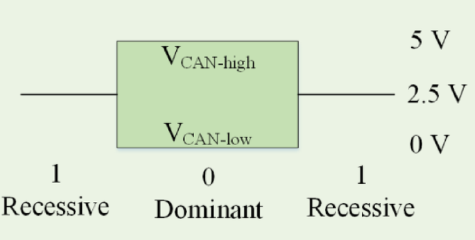
The signaling logic of a CAN bus.
In the protocol on the basis of message, each message has been recognized via a predetermined identifier instead of an address. A transmitted CAN architecture has been usually a protocol on the basis of message, so a message has been found to be a packet of data that aims to carry data. A message of CAN consists of 0 to 8 bytes of data arranged into a special network named an architecture. The data conceded per byte has been expressed within the protocol of CAN. Each node utilizing the protocol of CAN achieve an architecture, and CAN decides to accept it or not based on the node ID. If multiple nodes send the message simultaneously, the node with the highest priority gets access to the vehicle. On the other hand, low-priority nodes must wait until the vehicle becomes available.
link


