QKDTI A quantum kernel based machine learning model for drug target interaction prediction

This study proposed QKDTI – Quantum Kernel Drug-Target Interaction, a novel quantum-enhanced regression framework for DTI prediction that enhance the accuracy and efficiency of Drug-Target Interaction prediction. By leveraging quantum kernels, QKDTI captures complex molecular interactions more effectively than classical machine-learning approaches.

Traditional methods, such as classical ML and DL approaches, struggle with high-dimensional feature spaces, computational inefficiencies, and nonlinear interactions between molecular structures. SVR is a widely used machine learning technique for predicting continuous values, particularly in scenarios where the relationship between input features and output is complex and nonlinear. Traditional SVR relies on kernel functions such as linear, polynomial, and radial basis function kernels to project data into a higher-dimensional space where a linear regression model can be fit.

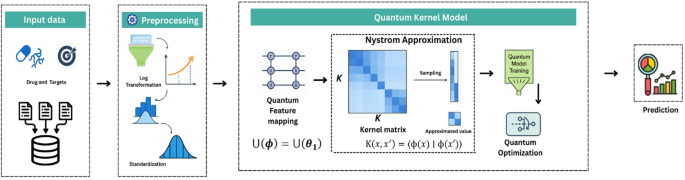
QKDTI provides an alternative approach by utilizing quantum kernels to map complex molecular interactions into higher-dimensional Hilbert spaces⁴³, capturing non-linearity more effectively than classical models. Unlike classical kernels, quantum kernels utilize quantum superposition and entanglement to capture intricate molecular structures and protein-ligand interactions more efficiently. This allows QKDTI to handle non-linearity in drug-target binding affinity predictions with improved precision. This study investigates the capability of quantum kernel learning for predicting binding affinity values in drug discovery applications. The methodology incorporates quantum-enhanced feature transformations with quantum machine learning techniques to optimize performance. The proposed framework consists of the following steps as shown in Fig. 1.

Dataset description

This study is based on datasets from the Therapeutics Data Commons: a widely used source of curated datasets for drug discovery³⁴. Among its extensive collection, three widely used datasets DAVIS, KIBA, and BindingDB were selected for training, testing, and validation of the proposed model. These datasets were retrieved using the TDC Python library interface, specifically from the multi-prediction DTI task module. Each dataset includes drug-target pairs along with their measured binding affinities, reported using experimental metrics such as Kd, IC50, Ki or integrated scores like the KIBA score.

Molecular Representations.

• Drugs – Small Molecules: Represented using SMILES – Simplified Molecular Input Line Entry System strings, a text-based encoding of molecular structure.

• Targets – Proteins: Represented using FASTA sequences, encoding the amino acid sequence of each protein target.

To prepare the raw molecular and protein data for machine learning models:

• Molecular fingerprints^44,45 or learned embeddings are derived from SMILES using RDKit cheminformatics tools.

• Protein features are extracted via pre-trained models or sequence-based descriptors like ProtBERT or physicochemical proper encodings.

Each dataset includes experimentally determined binding affinity values:

• DAVIS: Reports binding affinities in Kd (nM), specifically for kinase inhibitors.

• KIBA: Provides KIBA Scores, which are normalized affinity scores integrating multiple biochemical measurements.

• BindingDB: Includes a wide range of binding values reported as Kd, IC50, or Ki in nM, µM, or mM units.

The Binding affinity measurements and units are observed in Table 2.

Due to this wide scale in binding affinities from picomolar (pM) to millimolar (mM) raw values exhibit significant variance that could affect training stability.

Dataset composition

The chosen datasets vary in size, drug target pairs, and binding metrics, ensuring that the study covers a broad spectrum of drug-target binding prediction. The dataset characteristics are presented in Table 3.

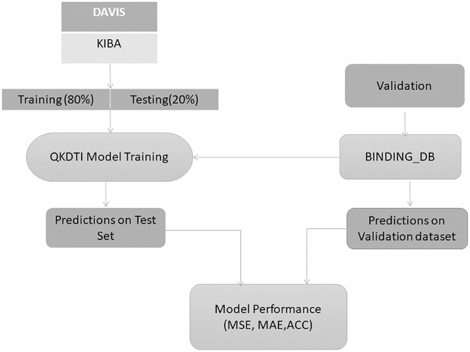
The DAVIS and KIBA datasets were used for training and testing in an 80:20 split, while the BindingDB dataset was employed exclusively for independent validation to assess the model’s ability to generalize to novel drug-target pairs can be observed in Fig. 2. To mitigate overfitting and ensure a clear evaluation of the model’s generalization capability, we deliberately limited the training and test datasets to subset samples. This controlled setting enables us to assess how well the model performs on unseen data. Datasets were selected because of their diversity, reliability, and relevance in drug discovery applications. These datasets are well-suited and standard for high-precision affinity models for DTI prediction. Exploratory data analysis has been done to reveal more molecular characterizations of the datasets.

Exploratory data analysis (EDA)

Exploratory Data Analysis (EDA) was conducted to understand the distribution and relationships among molecular descriptors, including molecular weight, lipophilicity (logP), hydrogen bond donors, and hydrogen bond acceptors, concerning binding affinity values.

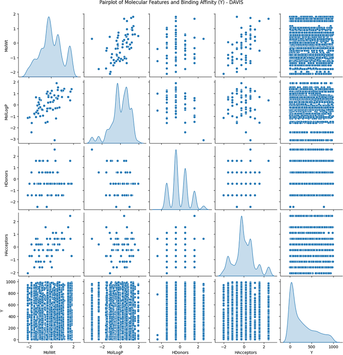
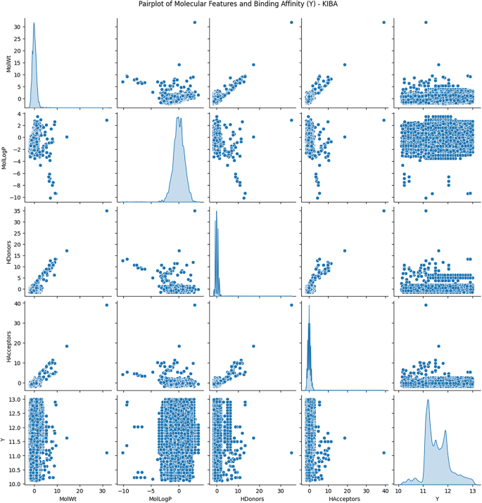
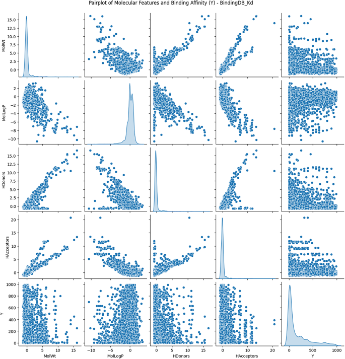
Figures 3 and 4, and 5 show the scatterplots of these descriptors across the DAVIS, KIBA, and BindingDB datasets, showing their distributions and pairwise correlations with binding affinity. These visualizations focus on how physicochemical properties influence interaction strength across different datasets. The observed variability in binding affinity, spanning from nanomolar (nM) to millimolar (mM) concentrations, necessitated logarithmic transformation to normalize the values and reduce variance during model training. This transformation enhances numerical stability and facilitates regression modeling.

Statistical analysis of datasets

To further understand the dataset properties, the log-transformed binding affinity values were subjected to statistical analysis. Table 4 presents the mean, standard deviation, and skewness for every dataset. Observably, the KIBA dataset shows the smallest variance (σ = 0.031) and maximum skewness and has a more uniform and right-tailed affinity score distribution, which are reasons for its higher model stability and performance. Conversely, BindingDB has the largest variance (σ = 1.372), implying a broader range of molecular interactions and higher complexity. The DAVIS dataset, while smaller, exhibits moderate variability and positive skewness, reflecting a prevalence of strong interactions with occasional weak binders.

These results demonstrate the non-linear, complicated nature of molecular descriptors vs. binding affinity, lending validity to the implementation of quantum-improved kernel learning within the QKDTI approach. The mapping of molecular attributes to a Hilbert space within quantum can enhance the ability of the model to capture the complexities of such relationships, allowing for better generalization and prediction performance.

Data preprocessing

The preprocessing phase is the critical step in developing a model. In this phase, it guarantees that the training and testing of the proposed model can be performed efficiently.

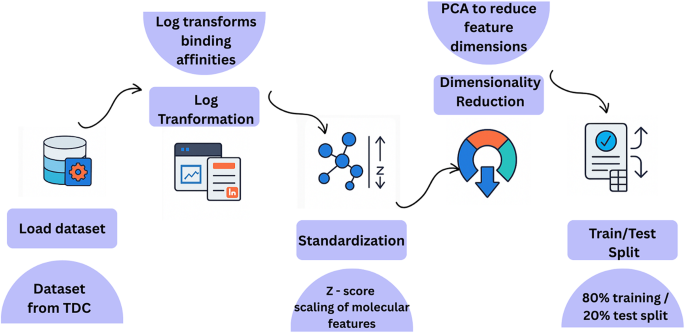
This process involves several operations shown in Fig. 6 applied to the DAVIS, KIBA, and BindingDB datasets, which serve as validation sets and contain diverse DTI pairs with varying binding affinity measurements. Due to the imbalance and heterogeneity of these datasets, feature transformation and standardization techniques were employed to maintain consistency across inputs and optimize model performance. At the outset, each of these datasets got its respective binding values from all data retrieved with ranges from nanomolar (nM) to millimolar (mM) concentrations. To normalize a vast extent of range, majorly fluctuating binding values were logarithmically transformed as:

Where Y represented the original binding affinity value, and Y_log described the transformed value of Y. This transformed log ensures that extremely large values would not dictate the learning trend while also providing variance stabilization for their multipurpose conformity towards regression models. Subsequently, to the transformation, standardization of features was performed using Z-score normalization, which scales each feature by subtracting the mean and dividing by the standard deviation as derived from the following:

Where X is the original value of the feature, µ is the mean across all instances for that feature while, σ is the standard deviation. This step was crucial in ensuring that no single feature disproportionately influenced the model, particularly when integrating quantum feature mapping techniques. To address missing values, a dataset-specific approach was taken. If any binding affinity values were missing, the corresponding data entries were removed. For missing molecular descriptors, the mean of the respective feature was used for imputation. Additionally, protein sequence embeddings were recomputed where necessary, ensuring a complete dataset for training.

Given the high-dimensional nature of drug and protein representations, principal component analysis was applied to reduce dimensionality while preserving 95% of the variance, making subsequent quantum computations more efficient. Finally, preprocessed datasets were then converted into a precomputed kernel format, enabling efficient training of the QKDTI model. These preprocessing steps ensured that the DAVIS, KIBA, and BindingDB datasets were well-structured and computationally optimized, allowing for seamless integration into the hybrid quantum-classical learning pipeline. This preprocessing framework improves numerical stability and facilitates effective comparisons between quantum kernel learning and classical techniques in DTI prediction.

Model development

In the previous section, the preprocessing pipeline was described to convert unstructured drug-target data to be built into a feature space suitable for machine learning models. Techniques including log transformation, standardization, quantum feature mapping, nyström kernel approximation, and feature fusion were applied to optimize learning conditions and enhance the model. Following data preprocessing, model training is performed. This section focuses on training strategies, optimization, and evaluation of QSVR meant for predicting drug-target binding affinities. The next steps should include an evaluation and training phase for several methods. This work aims to determine if the quantum-enhanced model provides explicit benefits in terms of accuracy, generalization, and computational efficiency. Already having outlined the details of the process including training with the QKDTI model, there are differences in contrast to classical models which do not rely on any manually developed kernels-either linear, polynomial, or RBF. Rather, QKDTI uses quantum feature mapping to produce kernels that exploit quantum entanglement and superposition to allow for a richer representation of data.

Quantum feature mapping

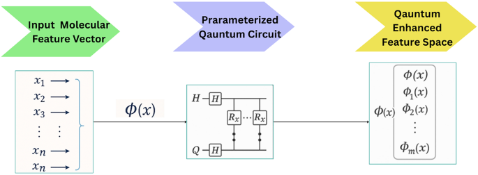
Once preprocessing was complete, the data was organized for quantum feature mapping, where molecular features were encoded into a quantum Hilbert space via parameterized quantum circuits (PQC)³⁴ can be observed in Fig. 7.

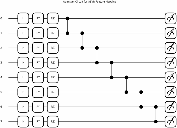
The quantum circuit used for QKDTI visualized in Fig. 8, consists of 𝑛 qubits corresponding to the molecular descriptor, which allows the embedding of high-dimensional molecular features into the quantum system. Each qubit is initialized in the standard basis state ∣0⟩. A Hadamard (𝐻) gate is applied on each of the qubits to attain the even distribution state, which allows for quantum parallelism:

This superposition allows the system to access multiple states of molecular features at once, boosting the model’s generalization capacity over different chemical structures. Once the Hadamard operation is performed, encoding of features is done using successive and parameterized rotation gates, namely the 𝑅𝑌 and 𝑅𝑍, which variably influence the qubit state from the descriptor value input given by the molecule. The transformation applied to each qubit is given by:

Here, \(\:{\text{x}}_{\text{i}}\) denotes the 𝑖th feature for the input molecular vector. These gates guarantee that the quantum amplitudes represent the molecular descriptors in a high-dimensional feature space. Controlled-Z (𝐶𝑍) gates couple adjacent qubits to introduce a dependence and correlation of features. The 𝐶𝑍 gate is defined as:

Here, it introduces correlations among phases across neighboring qubits, with a corresponding interaction angle that incorporates molecular interactions, which cannot be done by classical feature representations. The entanglement thus created ensures the quantum feature encoding captures complicated relations among molecular descriptors, finally enhancing the expressiveness of the quantum feature map.

Once the quantum feature encoding is complete, the expectation values of the quantum states are measured to compute the quantum kernel, which serves as the core of the QSVR model. The quantum kernel function was then computed using:

Here, 𝜙(\(\:x\)) represents a quantum-encoded transformation of the input features. Due to the exponentially rising computation complexity of the quantum kernel matrix for large datasets, a batch-wise computation strategy was adopted, splitting pairs into batches of 50 samples to ensure training efficiency. Besides, nyström approximation was additionally used to better improve computation efficiency and scalability to approximate the quantum kernel matrix.

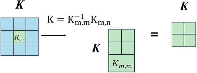
As shown in Fig. 9, the Nyström method permits approximation of large kernel matrices using a small set of landmark points, defined as follows:

Where \(\:{\text{K}}_{\text{m},\text{m}\:}\), which contains a subset of the full kernel matrix computed using a limited number of samples, and \(\:{\text{K}}_{\text{m},\text{n}}\) which gives the projection of the full dataset on these selected samples. By this approximation, the computational complexity is tremendously reduced, and at the same time, high accuracy concerning the actual kernel is retained.

Quantum optimization

Once the quantum kernel is calculated, it is used as an input to the QKDTI model and follows a standard epsilon-SVR optimization framework. The SVR objective function minimizes the following loss function.

Subject to the constraints.

w is the weight vector that the model learns. 𝜉𝑖 and 𝜉𝑖∗ allow small errors in predictions. 𝐶 controls the trade-off between accuracy and model complexity. 𝜖 sets the margin within which predictions are considered acceptable. This function helps QSVR find a balance between accuracy and generalization, preventing overfitting.

To train the QKDTI model effectively, we optimize various hyperparameters to achieve the best possible performance. The training process involves fine-tuning parameters that control the model’s complexity, computational efficiency, and generalization ability.

Hyperparameters

To optimize the performance of the QKDTI model, hyperparameters were carefully selected and tuned to ensure effective prediction.

Quantum circuit parameters

The quantum feature mapping in QKDTI utilizes eight qubits, each one representing a molecular descriptor. The qubits are put in a superposition state with Hadamard (𝐻) gates, then followed by parameterized rotation gates 𝑅𝑌(𝑥) and 𝑅𝑍(𝑥), which encode classical molecular feature values into quantum states. To introduce quantum entanglement and increase the correlation of the features, Controlled-Z (𝐶𝑍) gates were applied on pairs of adjacent qubits to exploit the complex interdependencies that can exist among molecular descriptors. The quantum circuit hyperparameters used in this study are represented in Table 5.

Quantum kernel approximation

To avoid kernel evaluations that would normally be found overpowering, the nyström approximation was adopted. This was achieved by picking out a batch of 50 to approximate the full kernel matrix, which would save on enormous costs while not significantly troubling the accuracy of the kernel. Furthermore, the double-batch computation considers 50 samples to be the batch during processing when ensuring extensive-scale kernel evaluation. The quantum kernels were fed to the SVR model when fitting it. SVR hyperparameters were thus jointly chosen for an optimal trade-off between model complexity and prediction accuracy. The hyperparameters related to the quantum kernel are outlined in Table 6.

Support vector regression (SVR) parameters

The regularization parameter (𝐶) was assigned a value of 1.0 to control the trade-off between efforts to minimize training error and maximize margin generalization. The epsilon (𝜖) parameter was set to 0.1, defining a tolerance range, with predictions inside that range being accepted as valid. The SVR model was fit using the Sequential Minimal Optimization (SMO) solver, which optimally solves the regression function. In the early stages of the modeling process, feature preprocessing is crucial to prepare input data for quantum embedding. In this study, PCA is used to reduce the dimensions of the features retained, accounting for 95% of the variance, so that only the most pertinent information is kept. In addition, Z-score normalization ensured that the molecular descriptors had a zero mean and unit variance before encoding them into quantum states. The SVR hyperparameters are provided in Table 7.

Optimal hyperparameter selection was essential for high predictive performance and low error rates. The Nyström approximation provided computational effectiveness without compromising the expressiveness of kernels. PCA-driven dimensionality reduction also enhanced generalization by reducing redundant molecular descriptors. Through the use of these optimizations, QKDTI showed substantial superiority over traditional models in binding affinity prediction on the DAVIS, KIBA, and BindingDB datasets.

Computational environment

The QKDTI model was implemented and tested using the following quantum-classical hybrid environment to ensure computational feasibility and performance evaluation.

Framework Used:

• Quantum Machine Learning: PennyLane.

• Quantum Backend: Qiskit for quantum kernel evaluations.

• Classical ML Libraries: Scikit-learn, PyTorch, TensorFlow.

Hardware & Execution Environment: