


Human breast cancer samples
Institutional ethics approval was obtained from the participating hospital institutions, University Health Network and Sunnybrook Hospital, both located in Toronto, Canada. The requirement for patients’ consent to use the breast cancer biopsy samples was waived by the ethics board due to the retrospective nature of the study and the anonymization of patient information.
Consecutive (sequentially identified without selection bias) ER+/HER2− invasive breast carcinoma diagnosed on core biopsies were identified from the institutional pathology database (N = 116 patients). Each sample contained between 1 to 3 tissue cores, resulting in varying size of imaged tissue areas. The luminal A cohort included 66 patients, while the luminal B cohort comprised 50 patients. The subset of patients who had clinical data useful for ML analysis was smaller (Nc = 68 patients), with 42 classified as luminal A and 26 as luminal B. The investigated clinical parameters were: Nottingham grade scores obtained from both the diagnostic biopsy and post-surgical resection specimens, primary tumour size, patient age at diagnosis, histologic subtype, number of lymph nodes with confirmed metastases, and number of sentinel (‘hot’) lymph nodes identified as suspicious and subsequently examined for metastatic involvement. Luminal A vs B classification of these samples was performed using genomic profiling (BluePrint® and MammaPrint®). Unstained 4.5 µm thick sections were prepared on charged microscope slides from FFPE (formalin-fixed, paraffin-embedded) tissue blocks that were used for the molecular assay. Minimal sample preparation involved chemical dewaxing to avoid potential polarisation imaging artifacts [25, 30,31,32]. No further processing was required for polarimetric imaging.
Polarimetric image acquisition and feature extraction
Mueller matrix (MM) imaging was utilised to capture the structural characteristics of unstained breast cancer biopsy samples, providing comprehensive polarisation data across the entire tissue section [23, 33]. Importantly, this method ensured full slide coverage without the need for pathologist-assisted (and thus somewhat subjective) ROI selection, allowing for an unbiased assessment of the tissue’s polarisation properties. For each biopsy, 24 polarimetric images were acquired using different configurations of the polarisation state generator (PSG) and polarisation state analyser (PSA), following the approach outlined by Tumanova et al. [23]. This image acquisition methodology increased the robustness and signal-to-noise ratio (SNR) of the polarimetric measurements [23, 33]. The experimental setup is illustrated in Fig. 2a, b.

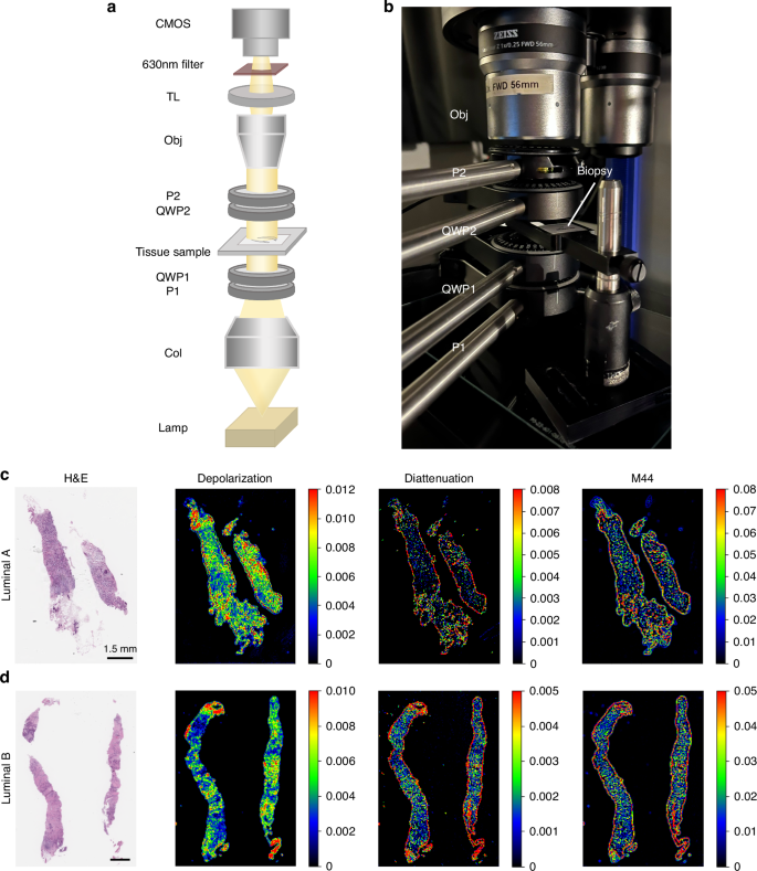
a Schematic of the Mueller matrix microscopy setup. Light from the source (Lamp) passes through a collimator (Col), a linear polarizer (P1), and a quarter-wave plate (QWP1) to form the polarisation state generator (PSG). After interacting with the sample, transmitted light passes through the polarisation state analyser (PSA; QWP2 and P2), a microscope objective (Obj), a tube lens (TL), a 630 nm filter, and is captured by a CMOS camera. b Photograph of the Mueller matrix microscopy system. c, d Representative polarimetric images of human breast core biopsy samples, showing H&E staining, depolarisation, diattenuation, and the M44 Mueller matrix element for luminal A (c) and luminal B (d) cases. Each image includes a 1.5 mm scale bar. Visual differentiation using these representative polarisation images remains challenging due to tissue heterogeneity, motivating the application of supervised machine learning; see text for details.
The polarimetric system consisted of a Mueller matrix polarimetry module integrated into a standard stereo zoom microscope (Axio Zoom V16, Zeiss) equipped with a Plan Neofluar Z 1X/0.25 NA objective lens. The PSG, which included a rotatable linear polarizer (LPVISE100-A, Thorlabs) and a rotatable quarter-wave plate (AQWP05M-600, Thorlabs), modulated the incident light polarisation, while the PSA, composed of the same elements but in reverse order, analysed the polarisation state of the transmitted light after interaction with the tissue. The microscope’s LED light source [Illuminator HXP 200C (D), Zeiss] emitted 310 W of uncollimated white light, which was passed through a filter centred at 630 nm (ET630/75 or ZET630/10, Chroma). Images were acquired using a Hamamatsu ORCA-Flash4.0 V3 Digital CMOS camera with a 2048 × 2048 pixel array and a pixel size of 6.5 × 6.5 µm². At a magnification of 7×, this setup provided a field of view of 18.9 × 18.9 mm² and an optical lateral resolution of 13.9 µm. The resolution was validated using a 1951 USAF resolution target (R3L3S1N, Thorlabs) [33]. To calibrate the system, we measured the input Stokes vectors at each pixel using a blank (air) sample, and subsequently calculated the output Stokes vectors with the reference samples (air and a retarder with known optical properties) in place [33]. This pixel-by-pixel calibration approach corrects for spatially dependent distortions arising from off-axis rays and ensures high spatial fidelity [33,34,35,36]. The system acquires 24 intensity images for different PSG/PSA configurations, enabling direct calculation of the Mueller matrix via Stokes vector formalism. While this exceeds the minimum 16-image requirement, the 24-image acquisition improves signal-to-noise ratio, enhancing overall data quality [31, 33,34,35,36]. In this study, calibration accuracy was considered acceptable when the difference between measured and theoretical Mueller matrices fell within a ~1–5% range.
Once the polarimetric images were acquired for the breast biopsy samples, pixel-by-pixel calculations of the Mueller matrix were performed using the Stokes formalism, as previously detailed [23]. From these matrices, key polarimetric parameters—depolarisation, retardance, and diattenuation—were extracted using the Lu–Chipman MM polar decomposition (MMPD), providing insights into tissue anisotropy and depolarisation [37]. In parallel, additional polarimetric parameters were derived using the Mueller matrix transformation (MMT), which complements the MMPD by characterising scattering and other structural tissue properties [38]. Both MMPD and MMT approaches are widely used in the bio-polarimetry research for detailed morphological analysis of biological tissues [18,19,20,21, 23]. The median value of each parameter was used as the representative metric for each slide, ensuring standardisation across samples regardless of the number of tissue cores present and the size of the surface area analysed from each patient [39, 40]. For consistency, all polarimetric parameters listed in the following sections thus refer to their median values across all pixels within each slide, unless otherwise specified.
The various derived polarimetric parameters offer biophysical insights into tissue microstructure, with a particular emphasis on the organisation and characteristics of birefringent structures, such as collagen [18,19,20,21]. For example, using the Lu–Chipman decomposition, parameters such as depolarisation (Δ), retardance (R), and diattenuation (D) were calculated, providing information about tissue scattering, fibre-related birefringence, and absorption anisotropy, respectively [18,19,20,21, 23, 37]. Additionally, the MMT parameters were employed to quantify the anisotropic properties of the tissue, including fibre alignment and birefringence [19, 20, 23, 38]. The 30 resultant polarimetric parameters were derived following the methodology outlined in previous studies [18,19,20,21,22,23,24], comprising 16 Mueller matrix elements, 8 MMPD, and 6 MMT metrics. A comprehensive list of these parameters is provided in Fig. 3.

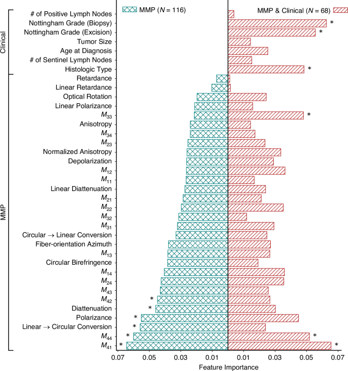
Features are Mueller Matrix polarisation (MMP) parameters and clinical variables as listed on the y-axis with their respective importance scores on the x-axis. Asterisks indicate the top six features contributing most to the classification models.
Machine learning methods
The classification task at hand necessitates a supervised ML approach, given the categorical nature of the problem (luminal A vs B). Feature selection through relative feature importance was undertaken as a preprocessing step to identify and select the most relevant features for improving model performance and interpretability. Then several established ML algorithms were considered, each offering distinct methodological advantages and trade-offs [41]. In this study, we systematically evaluated logistic regression (LR), linear discriminant analysis (LDA), support vector machine (SVM), random forest (RF), and extreme gradient boosting (XGBoost) to determine the optimal classifier for distinguishing between luminal breast cancer subtypes.
LR is a widely used method for binary classification, modelling the probability of an outcome using the logit function, which relates the log-odds of the outcome to a linear combination of the input features [41]. LDA, an extension of this approach, seeks to maximise class separability by identifying an optimal linear combination of features while assuming normally distributed data with equal class covariances [41]. SVM, a powerful kernel-based method, constructs a hyperplane that optimally partitions classes in a high-dimensional feature space, effectively handling complex decision boundaries [41]. RF, an ensemble-based approach, aggregates multiple decision trees to enhance predictive stability and mitigate overfitting, leveraging feature randomness to improve generalisability [41]. XGBoost, an advanced gradient boosting framework, iteratively refines decision trees by minimising classification errors through gradient descent, often achieving superior performance in structured biomedical datasets [42, 43].
Each method contains specific assumptions and design characteristics with varying applicability to the structure of the dataset used in this study. LR and LDA are computationally efficient and interpretable, though their assumptions may be limiting in datasets with non-linear boundaries or mixed feature distributions [41]. In particular, the assumption of equal covariances in LDA may not hold in the presence of heterogeneous clinical and polarimetric variables [41]. SVM does not assume any specific feature distribution and is flexible in modelling non-linear patterns, although its performance can depend on kernel selection and hyperparameter tuning [41]. Tree-based models such as RF and XGBoost are non-parametric, do not require feature normalisation, and are robust to multicollinearity and outliers. These properties make them applicable in settings with modest sample sizes, categorical outcomes, and potentially correlated features. However, these models are more complex and can be less transparent in their decision-making processes [41,42,43].
Handling outliers
Outliers were retained in the analysis, as no discernible clinical or biological rationale (e.g. age, ER/PR expression, lymph node status) justified their exclusion. While outlier removal is often employed to optimise machine learning model performance by refining decision boundaries and mitigating noise, its indiscriminate application risks eliminating biologically meaningful variability inherent in real-world clinical datasets [44]. Retaining these data ensures that the model is trained on a representative distribution, capturing the full spectrum of patient heterogeneity rather than overfitting to an artificially constrained dataset. Furthermore, excluding such cases may inadvertently bias the model by omitting rare but clinically significant phenotypes, ultimately compromising its generalisability and translational utility [44, 45].
Dataset partitioning and model training
Given the relatively small dataset, a 70% (train+validation)/30% (test) split ratio was implemented to optimise model learning capacity and generalisation. This partitioning strategy aims to train the model on a sufficiently large dataset while preserving an independent (not seen) test set for robust performance evaluation. To prevent class imbalance from skewing the model, stratified sampling was applied during data splitting, ensuring that the proportion of luminal A and luminal B cases remained consistent across all subsets [46].
To enhance model robustness and reduce the risk of overfitting, feature selection was performed as a preprocessing step using relative feature importance scores obtained from the random forest model [47]. RF was chosen for this task due to its ability to handle non-linear relationships, accommodate mixed feature types, and estimate variable importance directly during model training [41, 47]. This method ranks features based on how much they contribute to improving classification performance across the ensemble of decision trees. While alternative approaches to feature selection may yield somewhat different rankings, RF was selected to reflect the structure of our dataset, which includes potentially interacting polarimetric and clinical features [41, 47]. Subsequently, a five-fold cross-validation strategy (five different training-validation set combinations) was employed, whereby the 70% of the dataset was repeatedly partitioned into training and validation folds. Stratified sampling ensured class balance within each fold, and each sample contributed to both training and validation phases. This approach helps mitigate selection bias and provides a more reliable estimate of model performance under limited sample size conditions [48, 49].
Before final model testing, a retraining step was also conducted, where the best-performing model—selected based on training and validation results—was retrained on the combined training and validation set before being evaluated on the test (unseen data) set. This approach is widely used in machine learning, particularly in clinical datasets with limited sample sizes [50]. By incorporating additional (validation) data into the training phase, this method enhances statistical power and improves model generalisability without introducing data leakage, towards a more reliable estimate of real-world performance [50, 51].
Performance evaluation
To rigorously quantify classification performance on unseen data, a 2 × 2 confusion matrix (true subtype vs predicted subtype) was constructed. Standard classification metrics, including sensitivity, specificity, accuracy, and the area under the receiver operating curve (AUROC), were computed to provide a comprehensive evaluation of model effectiveness.
link