


Problem formulation
The task of data asset pricing fundamentally involves identifying patterns from complex observational samples to estimate the relationship between input features and asset price. In our setting, let \(S_S\in {!(M-}^{d}\) denote the \(i\)-th data asset instance, composed of structured and unstructured features, and let \({y}_{i}\in {\mathbb{R}}\) represent its corresponding price. Denote the input space as \(X=\{{x}_{i1},{x}_{i2},\cdots ,{x}_{id}|i\}\subseteq {R}^{d}\), and the label space as \(Y=\{{y}_{i}|i\}\subseteq R\). \(P(X)\) denotes an unknown probability distribution over X. The goal is to learn a pricing function \(f:X\to Y\), given a training dataset \(D={\{({x}_{i},{y}_{i})\}}_{i=1}^{N}\subseteq {(X,Y)}^{N}\).
Assuming that the mapping from X to Y lies within a hypothesis space H, the core task of data asset pricing is to learn a function \(\hat{f}\in H\) from the training data D, such that the expected error between predicted and actual values is minimized:
$$\hat{f}({x}_{i})=\mathop{\text{arg}\,\min }\limits_{\hat{f}({x}_{i})}{E}_{{x}_{i},{y}_{i}}(L({y}_{i},\hat{f}({x}_{i})))$$
(1)
Here, \(L({y}_{i},\hat{f}({x}_{i}))\) denotes the loss function. A smaller loss indicates a more accurate pricing model. In this study, we adopt the mean squared error (MSE) as the loss function.
Given the unknown and potentially nonlinear nature of the mapping between data features and prices, supervised learning models offer a principled approach to data pricing. By learning from labeled samples, they approximate the latent value function \(f\) that maps heterogeneous inputs—both structured and unstructured—to scalar price estimates. This allows the model to capture complex valuation patterns and support scalable, accurate pricing across diverse data assets.
Pricing framework
To better address the complexity of data asset valuation, we propose a multimodal pricing framework. It integrates structured indicators with unstructured textual descriptions to reflect the multifaceted nature of data value. As shown in Fig. 1, the framework consists of three main stages: data asset feature construction, integrated pricing, and scenario-based value assessment.

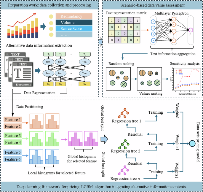
Data asset feature representation
In the first stage, both numerical and textual information are extracted to form a rich feature space for each data asset. The numerical side includes standard metadata such as data volume, redundancy, and rarity, which are quantified through statistical analysis. Meanwhile, the textual side focuses on functional descriptions (e.g., the content descriptions, use scenarios, and target consumers), which are processed using a pretrained language model (BERT) to generate dense vector representations. These heterogeneous features are integrated into a unified representation space, enabling the model to jointly leverage structured indicators and semantic attributes for pricing.
Integrated pricing module
Once features are constructed, the framework feeds them into a unified pricing module based on ensemble learning. Specifically, a LightGBM-based regressor is trained using both structured and unstructured features, and it performs global optimization by aggregating results from multiple locally learned regression trees. The model dynamically learns the mapping between multimodal features and observed prices, capturing complex interactions that traditional rule-based or linear models may miss. Furthermore, internal tracking of feature importance enhances interpretability and supports more accurate data pricing.
Scenario-based value assessment
To assess how different features influence pricing, the framework includes a scenario-aware evaluation component. Text features are first aggregated using multilayer perceptrons to preserve semantic information. Then, a ranking-based feature ablation is applied—features are sorted by importance and iteratively removed to assess their effect on model performance. This sensitivity analysis helps uncover which modalities and specific attributes contribute most to pricing accuracy, and provides actionable insights into the composition of data value.
Compared with traditional pricing frameworks, our design directly addresses two major challenges in data asset pricing: (i) how to systematically incorporate alternative (textual) data into the pricing process and (ii) how to model complex feature interactions without relying solely on handcrafted rules. This ensures that the framework is not only predictive, but also interpretable and adaptable to varied pricing scenarios.
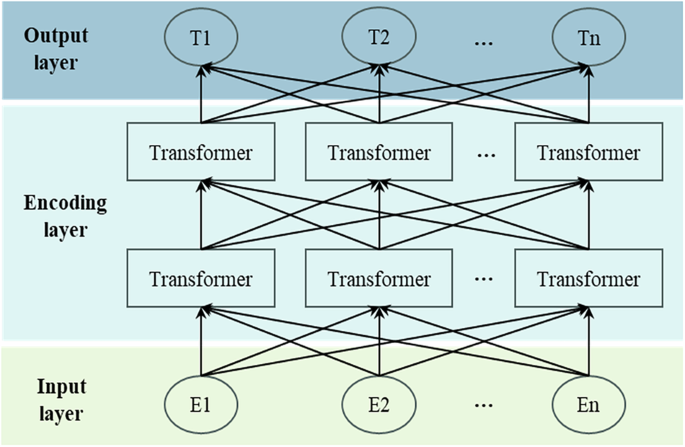
Bidirectional encoder representations from transformers
BERT is a pretrained language model designed to capture contextual semantics through a bidirectional Transformer encoder architecture. It computes dependencies between tokens using a multi-head self-attention mechanism, enabling it to learn rich semantic representations from unlabeled text corpora (Alonso-Robisco and Carbo, 2023). Its overall architecture, as depicted in Fig. 2, consists of an input layer, an encoding layer, and an output layer.

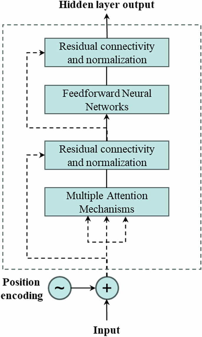
Each transformer block employs a multi-head attention mechanism, where embedded inputs are linearly transformed into Query, Key, and Value vectors. The structure of a typical transformer encoder is illustrated in Fig. 3, and its core computations are defined by Eqs. (2) to (4).
$$A{\rm{ttention}}(Q,K,V)={\rm{soft}}\,\max\left(\frac{Q{K}^{T}}{\sqrt{{d}_{k}}}\right)V$$
(2)
$$hea{d}_{i}=A{\rm{ttention}}(Q{W}_{i}^{Q},K{W}_{i}^{K},V{W}_{i}^{V})$$
(3)
$$MultiHead(Q,K,V)Concat(hea{d}_{1},\cdots ,hea{d}_{h}){W}^{o}$$
(4)
where the matrices \({W}_{i}^{Q}\), \({W}_{i}^{K}\), and \({W}_{i}^{V}\) are the respective weight matrices for Q, K, and V. The variable (i) denotes the number of attention heads, \({W}^{o}\) represents the mapping matrices of the multi-head attention mechanism.

In this study, BERT is applied to encode unstructured textual attributes of data assets—such as descriptions, functions, and usage contexts—into dense semantic vectors. These representations are later fused with structured indicators to form a multimodal input for the pricing model. The adoption of BERT allows the proposed framework to extract fine-grained contextual signals from domain-specific text, which enhances the model’s capacity to assess data value beyond what numeric indicators alone can reveal.
LGBM
LightGBM is an efficient gradient boosting framework based on decision trees (Sheng et al. 2024). It improves training speed and reduces memory usage by using histogram-based algorithms and gradient-based one-sided sampling (J. Hao et al. 2023; Yuan et al. 2023). These design choices allow it to scale effectively to large datasets with high-dimensional features.
The LightGBM algorithm is expressed as a summation function composed of k base models, as shown in Eq. (5).
$${\hat{y}}_{i}=\mathop{\sum }\limits_{t=1}^{k}{f}_{t}({x}_{i})$$
(5)
where \({x}_{i}\) denotes the input features of the i sample, \({f}_{t}\) represents the t base model, and \({\hat{y}}_{i}\) signifies the predicted value of the i sample. The loss function can be expressed in terms of the predicted and true values, as shown in Eq. (6).
$$L=\mathop{\sum }\limits_{i=1}^{n}l({y}_{i},{\hat{y}}_{i})$$
(6)
where n represents the sample size, l denotes the loss function of the i sample, and \({y}_{i}\) indicates the true value of the i sample. Based on these definitions, the objective function is formulated as shown in Eq. (7).
$$Obj(\theta )=\mathop{\sum }\limits_{i=1}^{n}l({y}_{i},{\hat{y}}_{i})+\mathop{\sum }\limits_{t=1}^{k}\Omega ({f}_{t})$$
(7)
where \(\Omega\) represents the regularization term, and \(\theta\) denotes the model parameters.
In this framework, LightGBM is employed to learn the mapping between multimodal features (textual and numerical) and the asset price. It is particularly well-suited for this task due to its ability to: (i) capture complex nonlinear relationships without requiring extensive manual feature engineering;
(ii) handle both sparse and dense features efficiently; and (iii) provide feature importance scores that enhance downstream interpretability (as utilized in section “LGBM”). By integrating LightGBM with the fused representations described in the section “Problem formulation”, the proposed model enables precise and scalable valuation of data assets in heterogeneous information environments.
SHAP
SHAP (SHapley additive exPlanations) is introduced to measure the importance of different data features. SHAP provides a unified framework that uses Shapley values to explain the predictive behavior of machine learning models. Shapley values, derived from cooperative game theory, represent the average marginal contribution of each feature (Jiang et al. 2024). Specifically, SHAP assigns importance values to each predictive feature based on an additive feature attribution method that adheres to a set of desirable theoretical properties: local accuracy, missingness, and consistency. The explanatory model associated with this method is shown in Eq. (8):
$$g(z^{\prime})={\phi }_{0}+\mathop{\sum }\limits_{i=1}^{M}{\phi }_{i}{z{\prime} }_{i}$$
(8)
where \(z^{\prime} \in {\{0,1\}}^{M}\) is defined as a joint vector indicating whether the i feature is present (=1) or absent (=0). M represents the total number of features, and \({\phi }_{i}\in {\mathbb{R}}\). In this approach, the explanatory model employs a simplified input \(x{\prime}\), which is mapped to the original input x via the mapping function \({h}_{x}(x{\prime} )=x\). This ensures that \(g(z{\prime} )\approx f({h}_{x}(z{\prime} ))\), where \(z{\prime} \approx x{\prime}\). The explanatory model is then established and trained to interpret the original model f. Given that SHAP measures feature importance by comparing the differences in model predictions with and without the feature, the SHAP value \({\phi }_{i}\) (i.e., the feature importance value) is calculated as the weighted average of all possible differences. This is expressed in Eq. (9):
$${\phi }_{i}=\mathop{\sum}\limits_{S\subseteq N\{{x}_{i}\}}\frac{|S|!(M-|S|-1)!}{M!}[{f}_{x}(S\cup \{{x}_{i}\})-{f}_{x}(S)]$$
(9)
where \(N\{{x}_{i}\}\) denote the set of features excluding \({x}_{i}\), and S represent the subset of features excluding the i feature. The predictions of the model with and without the i feature are denoted by \({f}_{x}(S\cup \{{x}_{i}\})\) and \({f}_{x}(S)\), respectively. It should be noted that SHAP becomes an additive feature attribution method only if \({\phi }_{0}={f}_{x}(\phi )\).
In the proposed framework, SHAP is applied to the trained LightGBM model to attribute the predicted price of each data sample to its multimodal features, with the prediction value expressed as the sum of individual SHAP values. This enables transparent interpretation of feature-level contributions and supports informed decision-making in data asset pricing.
link