Comprehensive input models and machine learning methods to improve permeability prediction

Data preparation
In the studied field, after collecting the required data, the information related to the logs of wells A and B was collected. The data were prepared in four stages: data loading, quality control and data editing, calculation of the required parameters before the main calculations and environmental corrections, and construction of the petrophysical model.
The primary goal of this research is to introduce diverse models that investigate various input data configurations. This study utilizes six main logs: gamma ray (GR), resistivity (RT), effective porosity (PHIE), density log (RHOB), sonic log (DT), and compensated neutron porosity (NPHI) logs. These logs, along with core data, serve as inputs for multiple machine learning methods, including the extreme learning machine (ELM), random forest regressor (RF), gradient boosting regressor (GB), support vector regression (SVR), and multilayer perceptron regressor (MLP). The six well logs were selected based on their common usage and significance in reservoir characterization and permeability prediction. Each of these logs provides essential information about different properties of the formation, contributing to a comprehensive dataset for machine learning models.
The objective is to achieve optimal permeability estimation by using the information provided by logs and core data. Each model, based on a specific machine learning method, is designed to accurately predict the formation permeability. The variety of models allows for a comprehensive exploration of different approaches to permeability estimation, considering the strengths and characteristics of each machine learning method.
The use of diverse models and input data configurations enhances the robustness of the study, providing a thorough analysis of permeability prediction in the studied field. This research aims to contribute valuable insights into the effectiveness of different machine learning approaches for permeability estimation, paving the way for improved reservoir characterization and management.
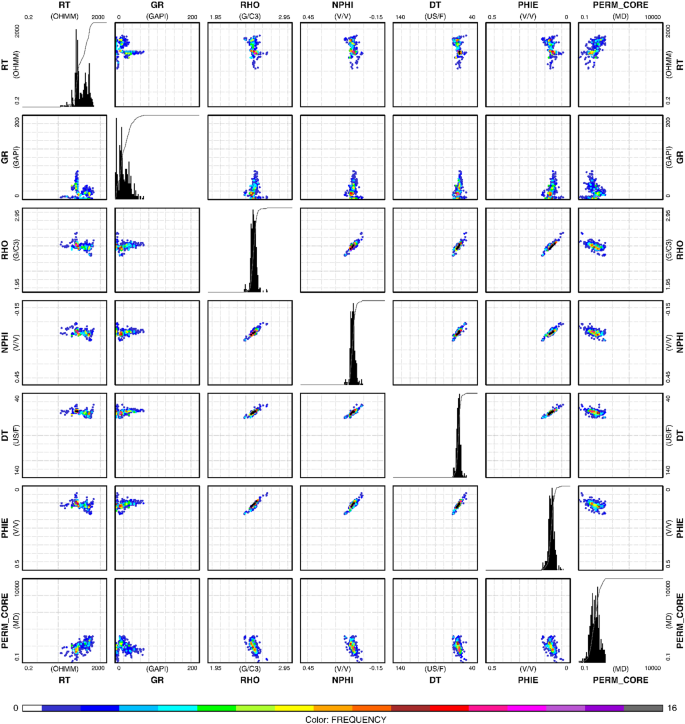
Each well in our study has a different number of data points. Specifically, Well A contains 86 data points of each desired well logs, and Well B contains 301 data points of each desired well logs, making a total of 387 data points across both wells. A summary of the input data is shown in Table 1.while Fig. 3 shows the linear relationships between the variables as well as their distributions.
In this study, Well C was utilized as a blind well to evaluate the effectiveness of the machine learning models. The data from Well C were not included in the training process of the models, ensuring that the models’ performance could be independently assessed. By using Well C as a blind well, the robustness and generalization capabilities of the models were tested, providing an unbiased evaluation of their predictive power. This approach helps in understanding the real-world applicability of the developed models and highlights their potential in accurately predicting permeability in unseen datasets.

Scatter plots of the variables against each other along with their distributions. The data frequency is shown according to the specified color bar from the lowest value in white color to the highest value in gray color. Key observations include strong correlations between RHO and PHIE, RHO and NPHI, RHO and GR, and NPHI and PHIE, indicated by tight clustering in the scatter plots. RT and PERM_CORE show weaker correlations with other variables. The histograms reveal that RHO and PERM_CORE distributions are highly skewed, with RHO concentrated at higher values and PERM_CORE peaking at lower values.
Data processing and performance metrics
Preprocessing is a crucial step in preparing data for training a neural network. Special functions were applied to both the inputs and outputs before training to enhance the efficiency of the network. The steps involved in this preprocessing include scaling the input and output data within a specific range, typically between 0 and 1. One reason for normalizing the data in this range is the behavior of activation functions, such as the sigmoid function, which may struggle to distinguish very large values. Normalizing the data helps address this issue and improves the training process. The process involves applying normalization functions before training and reverting them after the simulation. The specific equation or method used for normalization may vary, but it generally ensures that the data are transformed into a standardized range, making it more suitable for neural network training.
$$\:X_n=\fracX-X_minX_max-X_min$$
(4)
where \(\:X_n\) is the normalized data, \(\:\:X\) is the initial data, \(\:\:X_min\) is the lowest amount of data, and \(\:X_max\) is the highest amount of data.
The dataset was ultimately divided into three subsets: the training subset, the testing subset, and the validating subset. The distribution was 70% for training data, 20% for testing, and the remaining 10% for network validation. The choice of allocating a high percentage (70%) of training data is motivated by allowing the network to learn and adapt to the underlying patterns governing the input and outputs across various conditions.
The division was done randomly across all data (depth) points to ensure that each set contained a representative sample of the entire data range. This randomization helps in preventing any biases that could arise from sequential or depth-based ordering of the data.
During training, the network is exposed to the training data to adjust its parameters. Simultaneously, it is tested using the validation data to evaluate its performance and ensure that it generalizes well to new, unseen data. In the next step, various models were considered using six input logs, exploring each mode where these logs could be used as inputs together. This resulted in 57 different models representing permutations of two, three, four, five, and six input logs. These models were then employed to assess the degree of correlation and the impact of each input log on the permeability estimation. The goal was to obtain the best permeability estimation. The following five methods were used for all 57 models: extreme learning machine (ELM), random forest (RF), gradient boosting (GBR), K-nearest neighbor (KNN), and multilayer perceptron (MLP). The results from these models were recorded and analyzed to determine the effectiveness of each combination of input logs and regression algorithms for permeability estimation.
The next step involves comparing the 57 models to assess their performance. To effectively evaluate the proposed framework and conduct comparative studies with other models, common statistical qualitative measures are employed. Two key metrics used for this evaluation are the correlation coefficient (R2) and the root mean square error (RMSE).
Correlation coefficient (R2)
is a measure of the strength and direction of the linear relationship between the predicted and actual values. A higher value suggests better agreement between the predicted and actual values.
$$R^2=\frac\sum_i=1^n(y_i-y_mean)^2-\sum_i=1^n(y_i-y^\wedge_i)^2\sum_i=1^n(y_i-y_mean)^2$$
(5)
\(\:y_i\:\): Observed value.
\(\:y_mean\:\): Mean of observed values.
\(y^\wedge_i\): Predicted value.
\(\:n\:\): Number of observations.
Root mean square error (RMSE)
The RMSE measures the average magnitude of the errors between the predicted and actual values. It provides an indication of how well the model performs in terms of the absolute differences between the predicted and actual values. Lower RMSE values indicate better model accuracy.
$$\:RMSE=\sqrt\frac1n\sum_i=1^n(y_i-y^\wedge_i)^2$$
(6)
\(\:y_i\:\): Observed value.
\(\:y_mean\:\): Mean of observed values.
link


