Benchmarking machine learning methods for synthetic lethality prediction in cancer

Benchmarking pipeline
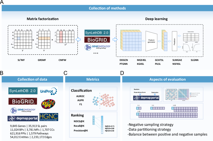
To evaluate machine learning methods for predicting SL interactions, we selected 12 methods published in recent years, including three matrix factorization-based methods (SL2MF31, CMFW32, and GRSMF33) and nine graph neural network-based methods (DDGCN34, GCATSL35, SLMGAE36, MGE4SL37, PTGNN38, KG4SL39, SLGNN40, PiLSL41, and NSF4SL42), see Table 1 for more details. The input data for these models varies, and in addition to SL labels, many kinds of data are used to predict SL, including GO28, PPI29, pathways30,43, and KG27, etc., and the detailed data requirements for each model are shown in Table 2. We believe that how many kinds of data inputs a model can accept is a function of the model’s own capabilities, and we focus on the model’s performance in various scenarios. To accomplish this, we designed 36 experimental scenarios, taking into account 3 different data splitting methods (DSMs), 4 positive and negative sample ratios (PNRs), and 3 negative sampling methods (NSMs) as shown in Fig. 1. In particular, these scenarios can be described as: (NSMN, CVi, 1:R), where N ∈ Rand, Exp, Dep; i ∈ 1, 2, 3; R ∈ 1, 5, 20, 50 (see Methods for specific settings). After obtaining the results of all the methods in various experimental scenarios, we evaluated their performance for both classification and ranking tasks, and designed an overall score (see Methods) to better quantify their performance in Fig. 2. We also evaluated the scalability of all the models, including their computational efficiency and code quality. In addition, we evaluated the impact of labels from computational predictions on model performance in Supplementary Notes 2.1, and included a comparison between KR4SL44 and several deep learning methods on a dataset processed according to KR4SL in Supplementary Notes 2.2. For a more visual presentation of the benchmarking results, we provided figures and tables (Fig. 2, Table 3, Supplementary Figs. 3–20 and Supplementary Data 1) to show the results under various scenarios.

A A total of 12 methods are compared, including 3 matrix factorization-based methods and 9 deep learning methods. B We collected data from different databases to build a benchmark dataset. C This study compared the performance of the models in both classification and ranking tasks. D We also designed various experimental scenarios, including different negative sampling methods, positive-negative sample ratios, and data partitioning methods. The combinations of these scenarios constitute a task space ranging from easy to difficult tasks.

A–C are the performance of the model under \(\rmNSM_\rmRand,\,\rmNSM_\rmExp\) and NSMDep, respectively, where lighter colors indicate better performance. The figure contains five parts of information: a) A list of the 12 models. b) The overall scores of the models and the combined scores under the classification task and the ranking task only. c) and d) The performance of the models under the classification and ranking tasks, including six experimental scenarios consisting of 2 DSMs and 3 PNRs. e) The average time required for the models to complete one cross-validation.
Classification and ranking
For the problem of predicting SL interactions, most current methods still consider it as a classification problem, i.e., to determine whether a given gene pair has SL interaction. However, models with classification capabilities alone are insufficient for biologists, who need a curated list of genes that may have SL relationships with the genes they are familiar with. This list can empower biologists to conduct wet-lab experiments such as CRISPR-based screening. Among the evaluated methods, only NSF4SL originally regards this problem as a gene recommendation task, while other methods belong to the traditional discriminative models. To compute metrics for both tasks using these models, we adjusted the output layer, this modification ensures that every model produces a floating point score as its output.
To assess the overall performance of the models in classification and ranking tasks, we employed separate Classification scores and Ranking scores (see “Methods”). Figure 2 presents these scores and the model’s performance across different scenarios and metrics. Based on the Classification scores, we found that when using negative samples filtered based on \(\rmNSM_\rmExp\), the models usually had the best performance for the classification task. Among them, SLMGAE, GCATSL, and PiLSL performed the best with Classification scores of 0.842, 0.839, and 0.817, respectively. On the ranking task, the models performed slightly better under the scenario of NSMRand, and the top three methods were SLMGAE, GRSMF, and PTGNN, achieved Ranking scores of 0.216, 0.198, and 0.198, respectively. From these scores, SLMGAE is the model with the best overall performance.
In the following three sections, for the purpose of consistently assessing the performance of each model across classification and ranking tasks, we have designated a single metric for each task. Given our focus on the accurate classification of positive samples and the imbalance between positive and negative samples in experimental settings, we primarily employ F1 scores to gauge the models’ classification performance. Additionally, to appraise the model’s effectiveness in the ranking task, we mainly rely on the NDCG@10 metric, which takes into account the relevance and ranking of the genes in the SL prediction list.
Generalizability to unseen genes
In this section, we utilized three different data splitting methods (DSMs) for cross-validation, namely CV1, CV2, and CV3 (see “Methods”), in the order of increasing difficulty. The performance of models given these DSMs reflects their ability to generalize from known to unknown SL relationships.
Among the three DSMs, CV1 is the most frequently used method for cross-validation. However, this method exclusively provides accurate predictions for genes present in the training set, lacking the ability to extend its predictive capabilities to genes unseen during training. The CV2 scenario can be characterized as a semi-cold start problem, i.e., one and only one gene in a gene pair is present in the training set. This scenario holds significant practical implications. Considering the existence of ~10,000 known genes involved in SL interactions, there is a substantial number of human genes remain unexplored. These genes, which have not yet received enough attention, likely include numerous novel SL partner genes of known primary genes mutated in cancers. CV3 is a complete cold-start problem, i.e., neither of the two genes is in the training set. Under CV3, the model must adeptly discern common patterns of SL relationships, to generalize to genes not encountered during training.
For the convenience of discussion, we fixed NSM to NSMRand and PNR to 1:1, i.e., our scenario is (NSMRand, CVi, 1:1), where i = 1, 2, 3. See Supplementary Data 1 for the complete results under all scenarios.
The left part of Table 3 shows the performance of the models under different DSMs while NSM and PNR are fixed to NSMRand and 1:1, respectively. From the table, it can be seen that, for the classification task, SLMGAE, GCATSL, and KG4SL performed better under the CV1 scenario, with F1 scores greater than 0.877. By contrast, CMFW and MGE4SL performed poorly, with F1 score less than 0.720. Under CV2, all the selected methods showed significant performance degradation compared to CV1. For example, the F1 scores of SLMGAE and GCATSL, still the top two methods, dropped to 0.779 and 0.775, respectively, while both of CMFW and MGE4SL decreased to less than 0.670. When the DSM is changed to CV3, only the F1 score of SLMGAE can still be above 0.730, while all the other methods drop below 0.700. For the ranking task, GRSMF, SL2MF, and SLMGAE exhibited better performance under the CV1 scenario with NDCG@10 greater than 0.270. However, under CV2, the NDCG@10 of almost all methods except for GCATSL and PTGNN are lower than 0.120. Lastly, when the DSM is CV3, the NDCG@10 scores of all the methods in this scenario become very low (lower than 0.010) except SLMGAE. Generally, SLMGAE, GCATSL, and GRSMF have good generalization capabilities. In addition, CV3 is a highly challenging scenario for all models, especially for the ranking task. However, it is worth mentioning that KR4SL has shown more promising performance compared to other methods in the CV3 scenario (see Supplementary Notes 2.2).
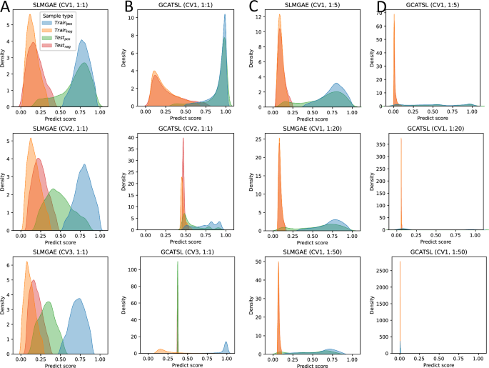
Moreover, Fig. 3A and B display the predicted score distributions of gene pairs in the training and testing sets for the SLMGAE and GCATSL models, respectively (see all methods in Supplementary Figs. 21–32). It is noteworthy that when the DSM is CV1, both models can differentiate between positive and negative samples effectively. As the challenge of generalization increases (in the case of CV2), there is a considerable change in the distribution of sample scores in the two models. In particular, for GCATSL, almost all negative sample scores in this model are concentrated around 0.5, while positive sample scores start to move towards the middle; for SLMGAE, only the positive sample distribution in the test set was significantly affected. When the task scenario becomes the most difficult CV3, the score distribution shift of the positive samples in the test set of the two models is more pronounced. For GCATSL, almost all sample scores in the test set are concentrated around 0.4, and the model cannot fail to have predictive ability in this scenario. Comparatively, SLMGAE is capable of distinguishing the samples in the test set with a relatively high degree of accuracy.

A, B are the scores of gene pairs in the training and testing sets for the SLMGAE and GCATSL models under various data splitting methods (DSMs). C, D are the score of gene pairs in the training and testing sets for the SLMGAE and GCATSL models under various positive and negative sample ratios (PNRs). The results are obtained with NSMRand.
Robustness to increasing numbers of negative samples
In our study, so far, all negative samples used in training have been screened from unknown samples. As such, there could be false negative samples among the gene pairs categorized as negative. This situation could inadvertently introduce noise into the model’s training process. Furthermore, given the substantial disparity between the numbers of non-SL pairs and SL pairs, these models encounter the issue of imbalanced data. To assess the robustness of these models to noise stemming from negative samples, we conducted experiments by gradually increasing the number of negative samples. In our study, the number of negative samples is set to four levels: equal to the number of positive samples (1:1), five times the number of positive samples (1:5), twenty times the number of positive samples (1:20), and fifty times the number of positive samples (1:50). Notably, the 1:1 ratio corresponds to the conventional experimental configuration frequently adopted.
In this section, our experimental scenario for comparison is denoted as (NSMRand, CV1, 1:R) where R = 1, 5, 20, 50. From the right part of Table 3, it can be seen that as the number of negative samples increases, the models’ performance (F1 score) in classification tasks gradually decreases. This phenomenon is particularly pronounced for CMFW and MGE4SL. When the number of negative samples increases from one to five times that of positive samples (PNR is 1:5), the F1 scores of CMFW and MGE4SL drop dramatically from around 0.700 to 0.531 and 0.335, respectively. By contrast, several other methods, namely SLMGAE, PTGNN, PiLSL, KG4SL, and GCATSL, maintain their F1 scores above 0.800. When the number of negative samples is further increased to twenty times the number of positive samples (PNR is 1:20), only SLMGAE achieved an F1 score above 0.800, while CMFW and MGE4SL dropped to 0.379 and 0.098, respectively. Finally, when the number of negative samples is fifty times that of positive samples (PNR is 1:50), SLMGAE still outperformed other models with an F1 score of 0.757, followed by SLGNN with an F1 score of 0.737. Notably, compared with previous PNRs, KG4SL and GCATSL experienced a significant decline in their F1 scores, dropping to 0.224 and 0.543, respectively. On the other hand, in the context of ranking task, when PNR = 1:5, SLMGAE, GRSMF, PTGNN, and DDGCN exhibited a slight improvement in NDCG@10 than PNR is 1:1. At PNR = 1:20, the NDCG@10 for SLMGAE, GRSMF, PTGNN, and DDGCN continued to rise. Lastly, the NDCG@10 values for SLMGAE and GRSMF continue to increase to 0.351 and 0.334, respectively, when the PNR is changed to 1:50. Generally, SLMGAE and GRSMF have stronger robustness.
Figure 3C and D display the distribution of the scores for positive and negative samples predicted by SLMGAE and GCATSL across different PNRs. The figure shows the impact of the number of negative samples on the score of the given gene pair evaluated by the models. As the number of negative samples increases, an increasing number of positive samples in the testing set are assigned lower scores. Despite this effect, the majority of samples are still correctly classified by SLMGAE. But for GCATSL, when the number of negative samples is twenty times that of positive samples, i.e., PNR = 1:20, almost all samples are assigned very low scores. When the PNR becomes 1:50, almost all the scores given by GCATSL are concentrated in a very small score range (around 0), and the predictions of the model are no longer reliable. Furthermore, under the results of SLMGAE, it is evident that the distribution of negative samples becomes increasingly concentrated with a higher number of negative samples. And a notable phenomenon is observed in the previous results (Table 3), that certain models exhibit improved performance in the ranking task as the number of negative samples increases. We hypothesize that this improvement is attributed to the higher concentration of scores among negative samples, resulting in a greater number of positive samples achieving higher rankings. Consequently, the performance of some models under ranking tasks improves with increasing PNR.
Impact of negative sampling
Obtaining high-quality negative samples is crucial for the performance of the models. However, in the context of SL prediction, high-quality negative samples are scarce. Therefore, it is important to explore efficient and straightforward methods for obtaining high-quality negative samples from unknown samples. In this study, we evaluated three negative sampling approaches, namely \(\rmNSM_{{{\rmRand}}},\,\rmNSM_\rmExp\), and NSMDep, which represents unconditional random negative sampling, negative sampling based on gene expression correlation, and negative sampling based on dependency score correlation, respectively (see Methods for details). Among these approaches, NSMRand has been widely used in existing SL prediction methods, and thus it will be used as the baseline for comparison. We denote the scenarios as (NSMN, CV1, 1:1), where N = Rand, Exp or Dep.
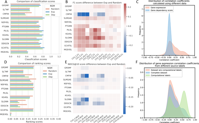
Based on the findings from the previous two subsections, certain characteristics regarding the model’s generalizability and robustness in the context of NSMRand can be observed. Here, we investigated two additional negative sampling methods (\(\rmNSM_\rmExp\) and NSMDep). Our observations revealed that models utilizing negative samples from \(\rmNSM_\rmExp\) demonstrate improved classification performance compared to NSMRand. On the other hand, models employing negative samples from NSMDep do not show significant performance differences relative to NSMRand (see Supplementary Data 1). The results of the classification and ranking tasks are presented in Fig. 4A and D. The majority of models demonstrate a marked improvement in the classification task when using \(\rmNSM_\rmExp\), with GCATSL’s Classification score increasing from 0.709 to 0.808. Other models such as SLMGAE, GRSMF, KG4SL, DDGCN, and PiLSL all achieved Classification scores above 0.720. On the other hand, SL2MF and CMFW experienced a decrease in performance. In the ranking task, the performance of NSMDep was better than \(\rmNSM_\rmExp\), but not as good as NSMRand. CMFW, DDGCN, and SLMGAE experienced a considerable decrease in their Ranking scores when using either NSMDep or \({{{{\rmNSM}}}}_{\rmExp}\), while the other models did not demonstrate a significant variation.

A, D show the overall score comparison of the models on the classification and ranking tasks under all three negative sampling methods (NSMs). B, E illustrates the differences between classification and ranking tasks using \({{{{\rmNSM}}}}_{{{{\rmExp}}}}\) and NSMRand in different scenarios, as measured by the F1 score and NDCG@10 metrics. Red and blue signify an increase and a decrease, respectively, with darker shades indicating a larger difference. C illustrates the distribution of correlation coefficients between known SL pairs of genes under different data sources. F illustrates the distribution of correlation coefficients between gene expression levels of SL pairs from different label sources.
We also assessed the impact of negative sampling on the generalization and robustness of the model. As shown in Fig. 4B and E, the negative samples obtained through \({{{{\rmNSM}}}}_{{{{\rmExp}}}}\) have a small impact on the performance of matrix factorization-based methods, except for the CMFW model, which has a significant decrease in performance in classification tasks compared to NSMRand. On the contrary, for deep learning-based methods, the negative samples obtained through \({{{{\rmNSM}}}}_{{{{\rmExp}}}}\) improve the classification task performance of the model in various scenarios, especially for the CV1 and CV2 scenarios. It is noteworthy that the performance of the NSF4SL model is not affected by the quality of negative samples, as it “does not use negative samples” (i.e., does not use negative samples at all) during the training process. For ranking tasks, except for CMFW and SLGNN, the quality of negative sample has a relatively small impact on most models.
Furthermore, we investigated the potential reasons underlying the different impacts of the negative sampling method. As shown in Fig. 4C, the distribution of gene expression correlation scores for known SL gene pairs exhibits a bias towards positive scores. Note that \({{{{\rmNSM}}}}_{{{{\rmExp}}}}\) selects gene pairs with negative correlation coefficient of gene expression. It is possible that, distinguishes the distribution of positive and negative samples in advance, reducing the difficulty of classification, it is able to because \({{{{\rmNSM}}}}_{{{{\rmExp}}}}\) improve the performance of the models in the classification task. By contrast, there is a symmetric distribution of correlation based on dependency scores, hampering the model’s ability to learn more effective features from the negative samples selected by NSMDep.
Impact of computationally derived labels on performance
Comparing Tables 3 and 4, it is evident that the performance of all the models across various DSMs generally improves significantly after excluding SL labels predicted by computational methods from the dataset (The complete results can be found in Supplementary Data 2). Of note, NSF4SL is elevated to the second best (i.e., runner-up) on the classification task, with F1 scores increasing by 0.108 and 0.135 in the CV1 and CV2 scenarios, respectively. Nevertheless, SLMGAE remains the best-performing model overall (see Supplementary Table 4). An explanation for the observed improvement in performance might be that, by filtering out the computationally derived SL labels, we have also reduced the noise in the model’s training data. Specifically for NSF4SL, which only relies on positive samples during training, the improvement in positive sample quality enables NSF4SL to achieve notably better ranking on dataset without computationally derived labels compared with complete dataset. We performed correlation analysis on gene expression within each of the three datasets: the complete dataset, the dataset excluding computationally predicted labels, and the dataset of solely computationally predicted labels. Results revealed that computationally predicted SL gene pairs predominantly clustered around the correlation coefficients of 0 and 0.5 (Fig. 4F).
Comparison with context-specific methods
In recent years, increasing attention has been paid to the prediction of context-specific SLs, leading to the development of methods such as MVGCN-iSL45 and ELISL46. To further assess the performance of machine learning methods in the context-specific settings, we benchmarked 7 models on cancer cell-line-specific data, including ELISL and MVGCN-iSL, along with the following 5 models which demonstrated superior performance among the 12 methods in the previous benchmarking study: SLMGAE, NSF4SL, KG4SL, PTGNN, and GCATSL. These 7 models were tested on 4 cancer cell lines: 293T (KIRC)47, Jurkat (LAML)48, OVCAR8 (OV)49, and HeLa (CESC)47,50. From the results, it is evident that SLMGAE performed particularly well on 293T and OVCAR8. NSF4SL performed the best on HeLa. MVGCN-iSL showed consistently competitive performance across all the cancer types except for 293T. ELISL’s overall performance was good but not highly competitive across the four cancer types. Detailed results can be found in Supplementary Notes 2.3.
link


