A proposed technique for predicting heart disease using machine learning algorithms and an explainable AI method

Figure 1 shows the proposed system’s sequences for predicting heart diseases. We first gathered and preprocessed the dataset to remove any necessary inconsistencies, such as replacing null occurrences with average values. We divided the dataset into two distinct groups, named the test dataset and the training dataset, respectively. Next, we implemented several distinct classification algorithms to determine which one achieved the highest accuracy for these datasets.

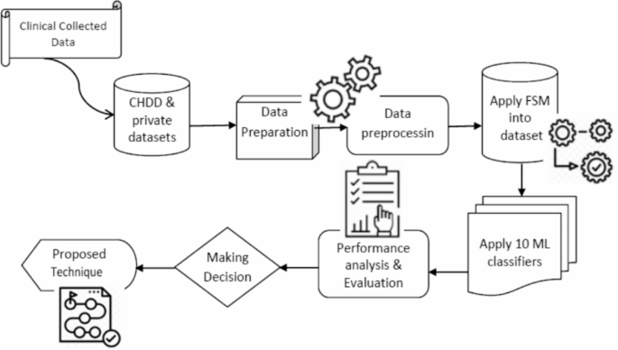
The proposed approach sequences for heart disease prediction.

The proposed methodology

This study investigates ML techniques such as Naive Bayes, SVM, voting, XGBoost, AdaBoost, bagging, DT, KNN, RF, and LR classifiers. These algorithms can aid doctors and data analysts in making correct diagnoses of cardiac disease. This article incorporates recent data on cardiovascular illness, as well as relevant journals, research, and publications. The methodology, as in¹, provides a framework for the suggested model. The methodology is a set of steps that transform raw data into consumable and identifiable data patterns. The proposed approach consists of three stages: the first stage is data collection; the second stage extracts specific feature values; and the third stage is data exploration, as shown in Fig. 1. Depending on the procedures employed, data preprocessing deals with the missing values, cleansing of the data, and normalization². We then classified the pre-processed data using the ten classifiers (A1, A2,., A10). Finally, after putting the suggested model into practice, we evaluated its performance and accuracy using a range of performance measures. This model developed a Reliable Prediction System for Heart Disease (RPSHD) using a variety of classifiers. This model uses 13 medical factors for prediction, among which are age, sex, cholesterol, blood pressure, and electrocardiography³.

Datasets and dataset features

This research employs both the CHDD and a private dataset for heart disease prediction. The CHDD dataset has 303 samples, while the private dataset has 200, and they have the same features. The combined dataset contains 503 records, and 13 features are associated with each one (including demographic, clinical, and laboratory parameters). The datasets have many features that can be used for heart disease prediction including age, gender, blood pressure, cholesterol levels, electrocardiogram readings-ECG, chest pain, exercise-induced angina, blood sugar with fasting condition, max heart rate achieved, oldpeak, coronary artery, thalassemia, and other clinical and laboratory measurements, as shown in Table 2. The outcome variable known as “Target” takes a binary value and refers to the heart disease predicting feature (i.e., it indicates whether or not cardiac disease is present).

Figure 2 shows the percentage distribution of individuals with heart disease in the combined datasets. A total of 503 samples have been gathered, and 45.9% of those have been diagnosed with HD, while the remaining 54.1% of individuals have not been infected with the disease.

Boxplots are an effective visualization technique for understanding the distribution of data and identifying potential outliers. By applying boxplots to a dataset related to HD, one can get insights into the distribution of a variety of HD-related features or variables. The HD dataset’s boxplots are illustrated in Fig. 3. Boxplots are used to illustrate the distribution of scores for HD detection in this figure. Every graph we obtained had an anomaly. Removing them will cause the median of the data to drop, which might make it harder to detect HD accurately. On the other hand, this method offers more benefits than the others; by identifying heart disease infection at an early stage, when medical care is most beneficial, this diagnostic could preserve lives.

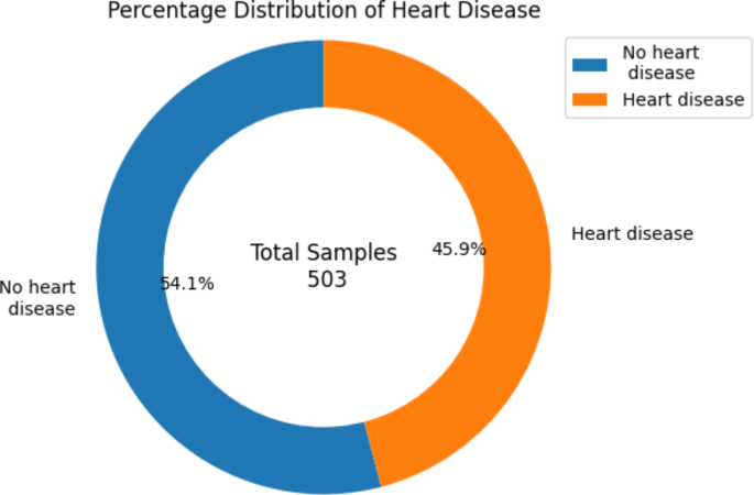
The percentage distribution of heart disease in the Combined dataset.

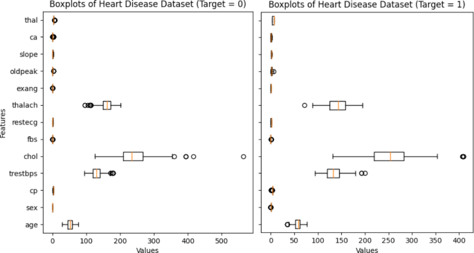
Boxplots of the combined heart disease dataset.

Dataset preparation

In this research, preprocessing was performed on collected data. The CHDD has four inaccurate CMV records and two erroneous TS entries. Incorrect data is updated to reflect the best possible values for all fields. Then, StandardScaler is employed to normalize all the features to the relevant coefficient, ensuring each feature has a zero mean and one variance. By considering the patient’s history of cardiac problems and following other medical concerns, an organized and composed augmented dataset was chosen.

The dataset studied in this research is a combination of accessible public WBCD and chosen private datasets. Partitioning the two datasets in this way allows us to use the holdout validation method. In this study, 25% of the data is in the test dataset, compared to 75% in the training dataset. The mutual information method is used in this research to measure the interdependence of variables. Larger numbers indicate greater dependency and information gathering.

The importance of features provides valuable insights into the relevance and predictive power of each feature in a dataset. Using this reciprocal information technique, the thalach feature is given the highest value of 13.65%, while the fbs feature is given the lowest importance of 1.91%, as illustrated in Fig. 4.

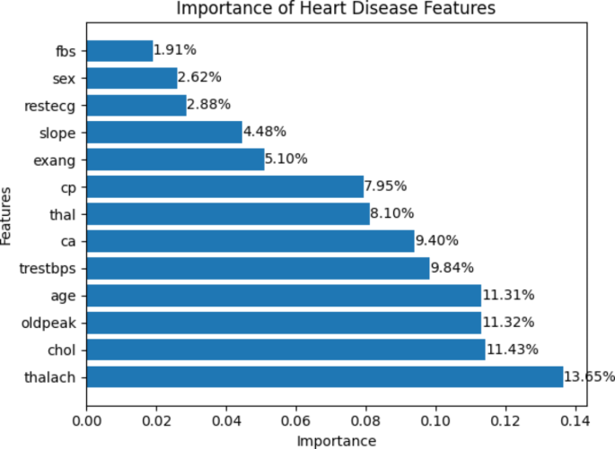
The importance of the heart disease dataset features.

Feature selection

In this research, we perform feature selection and classification using the Scikit-learnmodule of Python²⁰. Initially, the processed dataset was analyzed using several different ML classifiers, including RF, LR, KNN, bagging, DT, AdaBoost, XGBoost, SVM, voting, and Naive Bayes, which were evaluated for their overall accuracy. In the second step, we used the Seaborn libraries from Python to create heat maps of correlation matrices and other visualizations of correlations between different sets of data. Thirdly, a wide variety of feature selection methods (FSM) such as analysis of variance (ANOVA), chi-square, and mutual information (MI) were applied. These strategies are explained in Table 3 and are indicated by the acronyms FSM1, FSM2, and FSM3, respectively. Finally, the performance of several algorithms was compared for the identified features. The validity of the analysis was demonstrated using accuracy, specificity, precision, sensitivity, and F1 score. The StandardScaler method was used to standardize every feature before it passed into the algorithms.

The outcome of different feature selection methods

The F value for each pair of features is determined by using the ANOVA F value technique and the feature weights. Table 4(a) presents the findings of the ANOVA F test. The EIA, CPT, and OP features provide the most importance to the score, while the RES, CM, and FBS features contribute the least. Chi-square is another approach that determines the degree to which every feature relates to the target. Table 4(b) shows the chi-square outcomes. In this method, the first three features that are the most significant are MHR, OP, and CMV, whereas TS, REC, and FBS, respectively, are the least important ones. The MI technique is utilized in FSM3. To evaluate the degree of mutual dependency between features, this approach calculates the mutual information between them. A score of 0 indicates complete independence between the two features under consideration; a larger number indicates a greater dependence. The MI score results are shown in Table 4(c). CPT, TS, and CMV are the three features that are most dependent on each other in this case, whereas FBS and REC are the features that are independent of each other. Table 4 illustrates important factors that can be utilized for predicting the probability of having heart disease. Furthermore, REC, FBS, RBP, and CM all have lower total scores across all three FSMs. Because of all these features, three distinct groups are chosen to be included depending on their score. SF-1, SF-2, and SF-3 were the abbreviations that were given to each of the three different sets of features, respectively. Table 5 shows these feature sets that were selected for additional investigation.

Based on the research’s assessment of performance criteria (see Table 6), we chose the XGBoost classifier with SMOTE using the combined datasets and SF-2 feature subset. We will embed the most accurate technique in a mobile app and deploy the model using a variety of integrated development environments (IDEs), including Android Studio 14.0, Python 3.10, Spyder, Java 11, and Pickle 5²⁶.

The use of SMOTE and SHAP methods

To overcome the problem of imbalanced datasets, ML prediction applications employ the strong Synthetic Minority Oversampling Technique (SMOTE). This technique plays an important role in various applications.

1. 1.

   Balancing class distribution: In many prediction tasks, such as medical diagnosis and prediction, the dataset is often imbalanced. This implies that a particular class, typically the one of interest, has a lower representation than the other class. SMOTE interpolates minority class examples to create synthetic minority class samples. This balanced class distribution ensures the prediction model gets enough minority class examples to learn from.

2. 2.

   Improving predictive accuracy: In predictive modeling, an imbalanced dataset can cause the model to be biased towards the majority class, leading to poor performance in predicting the minority class. Accurate prediction of the minority class poses a significant challenge. Applying SMOTE trains the model on a more balanced dataset, improving accuracy and predictive performance, particularly for the minority class. This is critical in applications where missing the minority class (e.g., disease cases) can have significant consequences.

3. 3.

   Enhancing recall and precision: Predictive models trained on imbalanced datasets often exhibit high precision for the majority class but low recall for the minority class. This means they miss a large portion of the minority class instances, even if the ones they do identify are accurate. SMOTE helps improve recall without sacrificing precision, leading to a more balanced and effective model. In practical terms, this means the model is better at identifying all relevant cases, not just a select few.

4. 4.

   Reducing model bias: In prediction applications, a biased model can result in unfair outcomes, especially when the minority class is underrepresented. By exposing the model to a sufficient number of minority class examples during training, SMOTE mitigates this bias. This helps create a more equitable model that makes fairer predictions across all classes.

5. 5.

   Improving generalization: Models trained on imbalanced data may perform well on the majority class during training, but they fail to generalize well to new, unseen data, particularly for the minority class. By using SMOTE to create a balanced training set, the model is better equipped to generalize its predictions to new data, leading to more reliable and consistent performance in real-world applications.

6. 6.

   Enhancing robustness in deployment: In deployed machine learning applications, robustness is key. Predictive models often face real-world data that is skewed or imbalanced. SMOTE helps create a more robust model that can handle such data more effectively, reducing the risk of failure in production environments. This is crucial for applications like predictive maintenance, where identifying rare but critical failures can prevent costly downtime.

On the other hand, SHAP (Shapley Additive Explanations) is a powerful tool in ML that helps to interpret and explain the predictions made by complex models. The following are the benefits that SHAP offers in ML applications:

1. 1.

   Enhanced Transparency: SHAP makes black-box models more transparent, fostering trust among users and stakeholders. This is especially crucial in industries like finance, healthcare, and legal, where understanding model decisions is essential.

2. 2.

   Regulatory Compliance: Many industries are subject to regulations that require model decisions to be explainable. SHAP ensures compliance by providing clear, understandable explanations for each decision, facilitating documentation, and sharing with regulators.

3. 3.

   Improved user trust and adoption: When end-users understand why a model is making certain predictions, they are more likely to trust and adopt the technology. User interfaces can incorporate SHAP explanations to improve the user friendliness of AI-powered applications.

4. 4.

   Actionable Insights: SHAP doesn’t just explain predictions; it also provides actionable insights. For example, in prediction models, SHAP can identify key factors for effective features, allowing doctors to take proactive steps to detect disease.

5. 5.

   Facilitates Collaboration: SHAP explanations can bridge the gap between data scientists and non-technical stakeholders, facilitating better communication and collaboration. By providing a common understanding of model behavior, teams can work more effectively together.