A deep learning approach for line-level Amharic Braille image recognition

Due to the lack of publicly available datasets for our proposed solution, we prepared a custom dataset by collecting Amharic Braille documents.
Data set
We have collected Amharic Braille documentsfrom Addis Ababa university -Kennedy library. The documents include both typewritten and manually produced, most of which are typewritten and noisy. From different sized braille documents, this study uses the standard sized Braille, 11 × 11.5 inch, which is dominantly used in most centers, is selected6. As discussed in the literature, Braille documents may be one sided or double sided. For the reason that most Amharic Braille documents are single-sided6, the study is limited to single-sided Braille sheets. Details about the data set used in our study is described in Table 4 below.
A flat-bed scanner has been used for the digitization process. This is because it is the cheap alternative and easily available which can be used for so many other applications. The Braille document is scanned with a resolution of 200 dots per inch (dpi), which was used by most studies in Amharic braille document recognition. According to2, adequate spatial resolution setting should be between 80 and 200 dots per inch (dpi), if it is below 80 dpi, there is an insufficient amount of information and if above 200 dpi, the extra amount of information is superfluous.
For the variability of label sequences, the documents include the contents that deal for history of Ethiopia, law, agriculture and health. Furthermore, which are collected from real life degraded documents and scanned in low resolution (200dpi), for better training of the proposed solution. Each page has 28–29 lines, and there are 13 to 24 characters in each line image. Scanned braille documenta are transcribed into an equivalent Amharic document with line to line equivalence, by the help of visually impaired experts who can read braille documents. Finally 238 unique characters have been included in the dataset. Sample digitized brail document image and its equivalent Amharic text shown in Fig. 2 (part of the braille document page).


Braille Doc Image and equivalent text.
Skewness detection and correction of scanned document images is done by calculating the horizontal projection based on horizontal alignment of dots (cells). It is done on sobel filtered grayscale image to extract the bare bones (edges) to emphasize dots in the image by eliminating any noise. Horizontal projection array of the inverted image is implemented on sobel filter image at rotation angles between − 10 and 10. Then we have calculated the median of each projection array in each angle and pick the one which has the highest median, which is the angle of rotation that create bigger horizontal white regions. Finally we have rotated the image by this angle, which has highest median of horizontal projection array.
Text-line image segmentation
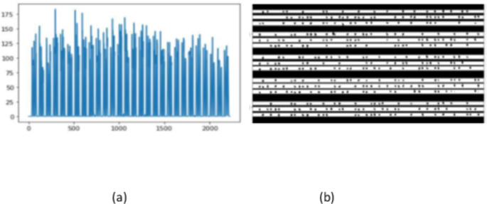
In this study line segmentation is also done by using Horizontal projection profile. Horizontal projection profile (HPP) is the array of sum or rows of a two dimensional image. Horizontal projection profile represented by lines (peaks) is equal to the number of lines on the document, where each line in the projection profile has a value that represents a number of black pixels in the corresponding row of the image as depicted in Fig. 3a, b.

As we can see in the Fig. 3, due to the horizontal space b/n dots in the cells of a line, lines of dots are grouped as one line. Based on the cropping region space difference between dots in the same cell and b/n cells of different lines, we could eliminate the separating regions between dots in the same cell. To do this, we have used a divider that can decrease these cropping regions from two directions to zero. I.e. regions = (np.max (hpp)-np.min (hpp)) /divider where (np.max (hpp)-np.min (hpp)) is the cropping space, hpp the calculated horizontal projection array and divider is the number that defines how much these regions should minimized in dimension.

Cropping regions for line images.
Figure 4a prescribes the regions where the cropping can pass in the binary images after their skewness was corrected. After that the Segmenting line used to separate into different line images is obtained by dividing the regions into two and getting the middle space of the region b/n lines obtained before as depicted in Fig. 4b. Finally, segmented line images are saved in grayscale with the .png file format, which is ideal for storing high-quality images that have been scaled down in size, making them smaller and more manageable, and are named with numbers beginning with 0001 and their equivalent line number in the label text.
Proposed model
The classical machine learning techniques ANN and other statistical classifiers such as Support Vector Machines (SVM), K-Nearest Neighbor (KNN), and Random Forests (RN) and so on, have been implemented for various applications. In recent years, deep learning has become the familiar technique, overshadowing the classical machine learning algorithms, due to its superior performance on wide ranges of tasks including speech, natural language, vision, and playing games.
Generally for processing of both spatially and temporally data like image captioning, question answering, and optical character recognition, researchers agree for using CNNs and RNNs in combination30. Accordingly, we have proposed a CNN-RNN hybrid model, which is illustrated in Fig. 5. In this framework, we employed three modules; CNN for feature extractor, RNN for sequence learner, and CTC as transcriber module. All three of these modules are integrated into a single framework and trained in an end-to-end fashion.

We have proposed a hybrid network model that is well adopted to spatio-temporal data problems. According to31, for image based (spatial structure) problems, CNNs are the best solutions and for sequence-based (sequential structure) data, RNNs are the most suited recognition32. The CNNs and RNNs are trained together in a supervised manner using braille line image and the corresponding ground-truth sequence of train dataset. At the top the Connectionist Temporal Classification (CTC) network is employed, which is responsible for alignment of output activations with the ground truth, error calculation, and transcription of the softmax prediction into labels. All these three modules are integrated into a single framework and trained in an end-to-end fashion, as illustrated in Fig. 6.
Sequence-to-sequence learning for OBR
Sequence-to-Sequence Learning is a means of training the model that is able to map an input sequence to an output sequence18,33. The use of CRNNs in combination with the CTC approach has gained significant traction for many sequence to sequence problems. This study focuses on employing a CTC-based sequence approach for Braille recognition, specifically avoiding segmentation and character-level alignment.
CTC in sequence learning
The connectionist temporal classification (CTC) is an algorithm introduced by Graves34 used for training RNNs such as Long Short-Term Memory (LSTM) networks, which enables end-to-end sequence learning by maximizing the probability of correctly recognizing sequences during training. This study34 describes a novel method for training RNNs to label unsegmented sequences directly, overcoming RNN’s requirements for pre-segmented training data and post-processing to convert their outputs into label sequences. Researchers conducted experiments on the TIMIT speech corpus, demonstrating its advantages over both a baseline HMM and a hybrid HMM-RNN.
For CTC-based sequence learning, the input is a sequence of observations, and the output is a sequence of labels with blank tokens as an additional output34. However Recurrent Neural Networks (RNNs) are great for processing sequential data, the output of a RNN needs a lot of post-processing to match it with appropriate labels, and that is where the Connectionist Temporal Classification (CTC) layer is able to help us for these applications. It transforms the outputs of the RNN into a conditional probability distribution over the possible label sequences. So CTC enables the output of the RNN to be directly usable without requiring additional pre or post processing steps. It tries all possible alignments of the Ground Truth text in the input and takes the sum of all scores, thereby making it alignment free.
The Ground Truth text is encoded in a special way to address problems related to duplicate characters and characters spanning across multiple time-steps. To handle the case of blank character at a time-step we use a special character and call it blank (-). When encoding a text, we can insert arbitrary many blanks at any position, which would be removed when decoding it. We can repeat each character as many times as we want. For a given Ground Truth alignment, the Neural Network outputs a matrix containing a score for each character at each time-step. The score for entire text is calculated by multiplying the corresponding character scores together. This gives us the probability of a particular Ground Truth alignment.
For a given training data D, x be an observation sequence of length T and y its label sequence of length L, the CTC objective function minimizes the negative logarithm of likelihood loss formulated as Eq. (1). The loss value is back-propagated through the Neural Network and the parameters of the Neural Network are updated according to the optimizer used.
$$\:\varvecL_\varvecC\varvecT\varvecC=-\varvecl\varveco\varvecg\left(\prod\:_(\varvecz,\varvecx)\in\:\varvecD\varvecP(\varvecz/\varvecx)\right)$$
(1)
where x = x1, x2, …, xT is the input sequence with length T, z = z1, z2, …, zC is the corresponding target for C < T and (x, z) ∈ D. p(πt/x) is computed by multiplying the probability of labels along the path π that contains output label over all time steps t as shown in Eq. (2).
$$\:\varvecP\left(\varvec\pi\:/\varvecx\right)=\prod\:_\varvect^\varvecT\varvecP(\varvec\pi\:_\varvect,\:\varvect/\varvecx)$$
(2)
where t is the time step and πt is the label of path π at t. CTC is independent of the underlying neural network structure rather it refers to the output and scoring.
There are many more observations than the actual labels. The last layer (softmax layer) of the network contains one unit per label that outputs the probability of having the corresponding label at a particular time step. There is a reduction function tell us ‘B’ used as mapping sequence of probabilities of observing a specific label (probability sequence from the network output of Soft-max) at a given time frame, into a predicted sequence y. Mapping is done by removing the repeated labels and then the blank predictions. The conditional probability of having a label sequence y given an observation sequence x is the sum of the probabilities of all paths π for which B (π) = y is obtained by the Eq. (3).
$$\:\varvecP\left(\varvecy/\varvecx\right)=\sum\:_\varvec\pi\:\in\:\varvecB\left(\varvecy\right)\varvecp(\varvec\pi\:/\varvecx)$$
(3)
For example, a sequence length observation (o), o = φeeφxφaφmmφpφleφ. Then, the paths are mapped to a label sequence as y = B (o) = B (φeeφxφaφmmφpφleφ) = B (φeφxφaφmφpφleφ) = ’example’, where B is a reduction mapping function which works by first collapse the repeated tokens and then remove blanks.
After the probability of label sequence y is obtained from an input sequence x with the CTC forward-backward algorithm proposed by34, we have employed the best path decoding method to find a character (C) that has the highest score from outputs (i) at every time-step and the final recognized string text could be generated without segmentation of the input sequence formulated as Eq. (4).
$$\:c_max=B\left(arg\underseti\textmax\left(y_i^t\right)\right)\textf\texto\textr\:\textt\hspace0.17em=\hspace0.17em1,\:2,\:3,\:\dots\:,\:\textT$$
(4)
link


