A deep learning framework with hybrid stacked sparse autoencoder for type 2 diabetes prediction

In the prediction of diabetes using the HSSAE algorithm, the research was conducted in three stages, as indicated in Fig. 1. Initially, the dataset was pre-processed using the Synthetic Minority Over-sampling Technique (SMOTE) in conjunction with min–max normalization. Following the pre-processing stage, the statistical analysis was performed to determine the nature of the data. Subsequently, the HSSAE algorithm was developed and trained with the pre-processed dataset. The HSSAE algorithm was employed to identify the complex patterns within the dataset, which were subsequently utilized for the prediction tasks. Finally, the performance of the algorithm, HSSAE, was evaluated using several metrics, including accuracy, precision, recall, F1 score, AUC, and Hamming loss. These metrics provided a comprehensive overview of the algorithm’s performance in diabetes prediction.

Framework of the study from data collection to evaluation.

Data acquisition, statistical analysis, and preprocessing

This study utilized the Diabetes Health Indicators Dataset (DHID), collected by the Centers for Disease Control and Prevention (CDC) via a telephone survey and available on Kaggle at “ The Health Indicator Dataset comprises 253,680 rows and 21 columns, with a sparsity of 43%, indicating that a substantial portion of the data contains zero values. Additionally, the EHRs Diabetes Prediction Dataset, accessible at “ was employed for diabetes prediction tasks. This dataset contains diverse patient information, including medical history, demographic data, and diabetes status, representing typical features of real-world clinical datasets. Initially, the dataset’s sparsity rate was 31%. To assess the robustness of the proposed HSSAE model under higher sparsity, we systematically increased the sparsity of selected numerical features (e.g., age, BMI, HbA1c level, and blood glucose level) by randomly setting 70% of their entries to zero, using a fixed random seed to ensure reproducibility. After this procedure, the sparsity of the selected features reached approximately 73%. The sparsity of each dataset was calculated using Eq. (1).

Statistical analysis of the sparse health indicators diabetes dataset

The dataset comprises two categories of variables: Numerical and Categorical. Numerical variables are quantitative measures such as Body Mass Index (BMI), general health, mental health, age, education level, and income, as presented in Table 2. BMI, with a mean of 28.38, high skewness (2.12), and kurtosis (10.99), highlights the presence of extreme obesity cases that are strongly linked to diabetes onset. General health, with a mean of 2.51, exhibits low skewness (0.42) and kurtosis (− 0.38), suggesting that most participants reported average health. Mental health (mean 3.18) and physical health (mean 4.24) show high variances (54.95 and 76.00) and strong positive skewness (2.72 and 2.20), indicating that while most individuals experienced minimal issues, a minority with severe conditions substantially affected the distribution. Age, with a mean of 8.03 and low skewness (− 0.35), reflects a well-balanced spread across groups, while education (mean 5.05) and income (mean 6.05) show negative skewness (− 0.77 and − 0.89), indicating that higher levels are more common, factors often associated with reduced diabetes risk. These patterns clearly highlight the significant impact of socioeconomic and lifestyle factors on determining health outcomes.

On the other hand, categorical variables provide qualitative insights that can be analysed through graphical representations, as shown in Fig. 2. The findings reveal clear associations between diabetes status and several health-related and lifestyle factors. Individuals with high blood pressure and high cholesterol are more likely to have diabetes. At the same time, those who regularly undergo cholesterol checks also show a higher prevalence, possibly reflecting underlying health concerns. Smoking, stroke history, and heart disease or heart attack are strongly associated with diabetes, highlighting their role as significant comorbidities. Conversely, engagement in physical activity and higher consumption of fruits and vegetables are associated with lower diabetes prevalence, suggesting a protective effect of healthy lifestyle behaviours. Heavy alcohol consumption shows a modest positive association with diabetes, whereas healthcare access and affordability (AnyHealthcare and NoDocbcCost) indicate that diabetes remains prevalent regardless of these factors. Furthermore, difficulty walking is highly correlated with diabetes, reflecting mobility challenges among individuals affected by the condition. Lastly, sex-based differences are observed, although diabetes is prevalent across both groups.

Categorical attributes of health indicator dataset.

Statistical analysis of the sparse EHRs diabetes prediction dataset

This dataset also comprises two categories of variables: The numerical features are Age, Hypertension, Heart disease, BMI, HbA1_level, and Blood_glucose_level, as shown in Table 3. Summarizes the statistical properties of the numerical variables in the diabetes prediction dataset. Age shows wide variability (mean 12.62, standard deviation 22.85) with positive skewness (1.62) and kurtosis (1.24), indicating a concentration of younger participants alongside fewer older individuals at higher risk. Hypertension (mean 0.07) and heart disease (mean 0.34) are rare, as confirmed by extreme skewness (3.23, 4.73) and high kurtosis (8.44, 20.40), which highlights the imbalance between affected and unaffected cases—a factor that can bias predictive models if not addressed. BMI (mean 8.20) shows mild skewness (1.17) and near-zero kurtosis (− 0.07), reflecting a relatively uniform spread. The HbA1c level (mean 41.18, standard deviation 2.60) demonstrates stable central tendencies with mild skewness (1.28), making it a reliable marker for diabetes. By contrast, the blood glucose level displays extreme variability (mean 0.86, variance 4501.92), with skewness (1.28) and kurtosis (0.29) indicating the presence of influential outliers. This heterogeneity reflects real-world metabolic dynamics, and while it challenges modelling, it provides critical diagnostic value.

On the other hand, Categorical variables offer qualitative insights that can be descriptively analysed using graphical representations to show the relationship between categorical variables, such as gender, smoking history, and diabetes status, as shown in Fig. 3. As observed, diabetes cases are significantly limited among males and females, with the “Other” gender category contributing very few instances. This may be due to their underrepresentation in the data. For smoking history, individuals with no history of smoking or those who never smoked form the highest proportion in both diabetic and non-diabetic groups. However, a substantial number of diabetes cases also occur among former and current smokers, indicating an association between smoking status and the risk of diabetes. The “ever” and “not current” categories are relatively lower-case numbers, indicating lower prevalence or reduced reporting.

Categorical attributes of the ehrs diabetes prediction dataset.

Data pre-processing

Before applying the proposed algorithm, the datasets were divided into training and testing sets, with a 70:30 split to ensure adequate model training while preserving data for validation⁴³. To guarantee reproducibility, this split was performed using a fixed random seed (random_state = 42). Normalization was applied using the MinMax Scaler to ensure that all features contribute equally. The min–max normalization approach provided in Eq. (2) was used to scale the feature values into the range [0, 1]⁴⁴.

where \({X}{\prime}\) = normalized value,\(X=\) original value, \(\text{min}(X)\) = minimum value of \(X\), and max \((X)\) = maximum value of X. It was observed that the datasets contained only a limited number of positive samples, while the majority were negative, resulting in a biased class distribution. To address class imbalance, the Synthetic Minority Oversampling Technique (SMOTE)⁴⁵ was applied with a fixed random state (random_state = 42) to ensure reproducibility. SMOTE generates new instances of the minority class by sampling the feature space of each target class and its nearest neighbours, creating synthetic examples while preserving the characteristics of the original dataset⁴⁶. After applying SMOTE, the classes were balanced, as shown in Table 4, resulting in more reliable predictions and reduced bias when training ML and DL models.

Methodology

An autoencoder (AE) is a type of unsupervised neural network with three layers⁴⁷, including an input layer, a hidden layer, and an output layer (reconstruction), as given in Figs. 4 and 5 illustrates its model representation. The autoencoder can gradually convert artificial feature vectors into conceptual feature vectors, effectively performing a nonlinear transformation from a high-dimensional space to a low-dimensional space. The automatic encoder’s operation consists of two main stages: encoding and decoding.

Autoencoder model representation⁴⁸.

The proposed HSSAE model

In this study, the HSSAE algorithm was developed, as shown in Fig. 6. All the processes were presented before the classification results were obtained.

Flowchart of proposed algorithm HSSAE.

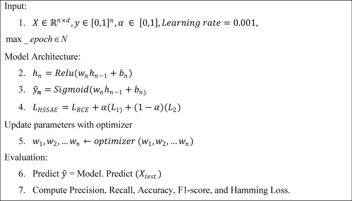
The sequential breakdown of the flow chart in Fig. 6:

Unified architecture

The HSSAE algorithm is based on the SSAE principle, as shown in Fig. 7. However, SSAE focuses on the reconstruction-based features. SSAE expect the decompression-reconstructed output data \(\widehat{X}\) to restore the input data \(X\) as much as possible, i.e., \(\widehat{X}\approx X\). Suppose the input data \(X=\{{x}_{1}, {x}_{2}, {x}_{3},\dots .{x}_{l}\}\) are the training samples of size \(l\), each set of samples has \(N\) observations \({X}_{i}= {\{ {x}_{i,1}, {x}_{i,2}, {x}_{i,3},\dots .{x}_{i,N}\}}^{T},X\in {\mathbb{R}}^{N\times L}\) then \(\forall i=1, 2, 3, \dots .l,\) then the loss function of stacked sparse autoencoder as represented in Eq. (3).

where the first term \(\frac{1}{m}\sum_{i=1}^{m}\frac{1}{2}{\Vert \widehat{{X}_{i}}-{X}_{i}\Vert }^{2}\) of Eq. 3, called the Mean Squared Error (MSE), measures how accurately the network reconstructs the input data. The second term is called \({L}_{2}\) norm that penalizes the large weight values. This term helps the model prevent overfitting by encouraging smaller, more generalized weights. The parameter \(\lambda\) controls the strength of this penalty. The third term \(KL\left(\rho \parallel {{\rho }{\prime}}_{h}\right)\) is called the Kullback–Leibler (KL) divergence, which enforces the sparsity in hidden layers of the network. Sparsity ensures that only a small subset of neurons is activated at a time. The KL divergence quantifies the difference between the desired average activation level \((\rho )\) and the actual activation \({{\rho }{\prime}}_{h}\) of the hidden layer neuron. The parameter \(\beta\) control the sparsity constraint. The SSAE extracts features from the data and applies an ML model for classification. However, SSAE faces two challenges, i.e., neglecting the discriminative features of learning for sparse data prediction⁴⁹. Additionally, using latent space with another algorithm, i.e., an ML model for prediction, increases the computational complexity⁵⁰.

To address the limitations of the SSAE and HSSAE, a custom hybrid loss function has been proposed, where the HSSAE algorithm integrates a supervised classification layer, i.e., sigmoid, into the latent space of the encoder and passes the decoder part. Several important components of the HSSAE algorithm, which are crucial for the entire learning process, are given below.

Encoder layer

The encoder layers of the HSSAE algorithm map the input data to a lower-dimensional latent space representation. Many nonlinear transformations within these layers learn to extract the most prominent features and patterns. Let \({X}_{input layer}={h}^{0}\) represent the input layer, then the encoded layer can be defined by Eq. (4).

where, \({h}^{l}\) is the output of the \({l}^{th}\) layer, \({w}^{(l)}\) is the weight matrix of \({l}^{th}\) layer, \({h}^{(l-1)}\) is the output of the previous layer \({(l-1)}^{th}\), \({b}^{l}\) is the bias vector of the \({l}^{th}\) layer and \(\sigma\) is the activation function, i.e., ReLU.

Latent space layer

The latent space layer, as shown in Fig. 8, contains the most important and instructive features from the input data, removing noise and unnecessary information. Typically, the autoencoder follows the path of an encoder, a latent space, and a decoder on the input data to make predictions.

Proposed algorithm HSSAE structure.

Binary prediction needs a feature in an extracted form, and any classification model or layer can be applied to perform it. The latent space layer can be mathematically represented in Eq. (5).

where \({Z}_{Latent}\) represent the latent representation of the input data and \({h}^{(L)}\) is the output of the last layer.

HSSAE classification layer

The HSSAE algorithm utilizes the features extracted in the bottleneck layer directly for classification by applying a sigmoid layer, rather than decoding the latent representations, as illustrated in Fig. 9. This approach significantly reduces computational complexity while optimizing the prediction task. Unlike SSAE, the HSSAE algorithm employs the learned latent representations for classification without requiring an additional ML classifier. The output of the last encoder layer \({h}^{(L)}\), is passed through a sigmoid activation function \(\varphi\), to obtain the predicted probabilities \(\widehat{y}\) for binary classification, as defined in Eq. (6) and (7):

Proposed algorithm HSSAE with classification layer.

The HSSAE algorithm generates probabilities in the range [0, 1] for each instance, which can serve as a simple measure of predictive confidence: values close to 0 or 1 indicate high confidence. In contrast, values near 0.5 indicate higher uncertainty.

In a binary classification problem, \(\widehat{y}\) is the probability predicted by the model that this input belongs to the positive class. Due to the sigmoid activation function \(\varphi\) the output is constrained between 0 and 1, which also provides a probabilistic interpretation of how much the model considers in its prediction. The HSSAE algorithm combines supervised classification and unsupervised feature learning in a single framework, showing effectiveness through the integration of the encoder and classification layers in using latent representations. This will enhance the model’s ability to simplify predictions of target variables and strengthen its capacity to extract relevant features.

\({\mathbf{L}}_{1}\)regularization

\({\text{L}}_{1}\) Regularization, also referred to as Lasso regularization, modifies the loss function by adding the total of the model’s coefficients’ absolute values. This method successfully performs feature selection while promoting sparsity by adjusting some coefficients to absolute zero. As a result, the model might ignore characteristics that are less important or irrelevant. \({\text{L}}_{1}\) regularization is useful for high-dimensional datasets where feature selection is crucial. The \({\text{L}}_{1}\) regularization term can be stated mathematically as given in Eq. (8).

where \(\alpha\) is the regularization parameter, \({w}^{l}\) denotes the weight matrix of the \({l}^{th}\) layer, and \({\Vert {w}^{l}\Vert }_{1}=\sum_{ij}\left|{w}_{ij}^{(l)}\right|\), represents the \({l}_{1}\)-norm, calculated as the sum of the absolute values of all coefficients in the weight matrix.

\({\mathbf{L}}_{2}\)regularization

\({\text{L}}_{2}\) Regularization, also known as Ridge regularization, adds the squared values of the model’s coefficients to the loss function. Unlike \({\text{L}}_{1}\) regularization, \({\text{L}}_{2}\) regularization favours small coefficients rather than forcing them to be exactly zero. This reduces overfitting by spreading the effect of a single feature across numerous features. \({\text{L}}_{2}\) regularization is very beneficial when input characteristics are correlated. The \({\text{L}}_{2}\) regularization term is stated mathematically as given in Eq. (9).

where \(\alpha\) is the regularization parameter, \({w}^{l}\) denotes the weight matrix of the \({l}^{th}\) layer, and \({\Vert {w}^{(l)}\Vert }_{2}^{2}=\sum_{ij}{\left({w}_{ij}^{(l)}\right)}^{2}\) represents the squared \({l}_{2}\)-norm, calculated as the sum of the squares of all coefficients in the weight matrix.

Like \({\text{L}}_{1}\) regularization, \(\alpha\) is the regularization parameter, whereas \({w}^{l}\) represents the model coefficients. The total is calculated for all coefficients, and the squares of the coefficients are added.

Binary cross-entropy (BCE)

The objective of binary classification tasks, such as predicting diabetes, is to learn the probability that a given dataset belongs to one of two groups. The model makes binary predictions by approximating the probability using the BCE loss function, as shown in Eq. (10), which measures the difference between class labels and predicted probabilities. BCE is well-suited for binary classification since it complements the sigmoid activation function, whose outputs range from 0 to 1. BCE is also differentiable and can therefore be used with gradient-based optimizers, such as Adam, which can lead to effective model training. BCE also provides a probabilistic output of prediction, which can be used in medical diagnosis and many other applications where the model’s confidence can contribute towards decision-making.

where \(y\in \{\text{0,1}\}\) is the actual binary label and \(\widehat{y}\in [\text{0,1}]\) is the predicted probability.

Custom hybrid loss

The objective of the HSSAE algorithm, is not only to preserve the reconstruction capabilities but also to optimize the model for task-specific predictions, making it particularly effective for sparse data scenarios. However, minimizing the MSE reconstruction-based optimization in SSAE fails to extract essential features for downstream predictive tasks. Moreover, the \(KL(\rho \parallel {{\rho }{\prime}}_{h})\) does not adapt well to datasets with uneven sparsity patterns, where certain features or data dimensions may dominate others. To address these limitations, in this study, a custom hybrid loss function is developed that incorporates the BCE loss function and a dynamic and finely tuned balance between the sparsity-inducing \({\text{L}}_{1}\) norm and the stability-enhancing \({\text{L}}_{2}\) norm. This exceptional formulation, \(\left({L}_{1}\right)+(1-\alpha ){\text{L}}_{2}\), where \(\alpha\) range from \(0\le \alpha \le 1\) is not just a mathematical adjustment; it is a groundbreaking approach for tailoring the model’s performance to the specific challenges posed by sparse, high-dimensional datasets. By assigning a weight of \(\alpha\) to the \({L}_{1}\) norm, the hybrid loss function actively encourages sparsity, driving less relevant coefficients to zero and enabling effective feature selection. Simultaneously, the complementary \((1-\alpha )\) the weight allocated to the \({\text{L}}_{2}\) norm ensures stability by reducing large coefficients, distributing influence evenly across features, and enhancing the model’s generalization ability. This interaction provides unparalleled flexibility: a higher \(\alpha\) sharpens that focuses on essential features by prioritizing sparsity, while a lower \(\alpha\) Stabilizes the learning process and reduces sensitivity to noise by emphasizing smooth optimization. The following hybrid loss function is optimized using the HSSAE algorithm to accomplish these two goals, as shown in Eq. (11)

Putting the values of \(\left({E}_{B.C}\right), ({L}_{1})\) & \(({L}_{2})\) in Eq. 11, as given in Eq. (12).

Here, \({E}_{HSSAE}\) denotes the hybrid loss function, \(\alpha \in [\text{0,1}]\) controls the balance between sparsity \({(l}_{1})\) and weight shrinkage \({(l}_{2})\), \({w}^{\left(l\right)}\) are the weight matrices of the \({l}^{th}\) layer, and \(\text{log}\) denotes the natural logarithm. The ideal weights and biases are obtained through greedy layer-wise pretraining, followed by fine-tuning with backpropagation, which minimizes the hybrid loss to align the network’s outputs with the target predictions. The gradient of the hybrid loss with respect to the weight matrix \({w}^{\left(l\right)}\) is expressed in Eq. (13)

where \(sign(\cdot\)) denotes the sign function, defined as \(sign\left(x\right)=-1\) if \(x<0\), \(sign\left(x\right)=0\) if \(x=0\) and \(sign\left(x\right)=1\) if \(x>0\). Consequently, Eqs. (14) and (15) represent the weight and bias update processes.

where \({w}^{(l)}\), \({\text{b}}^{(l)}\) are the weight and bias, and \(\mu\) represents the learning rate. Traditional gradient descent methods, such as Stochastic Gradient Descent (SGD) and Mini-Batch Gradient Descent, apply a uniform learning rate across all network parameters. This approach can be limiting, particularly in sparse datasets like those handled by the proposed algorithm HSSAE, which often contain rare or less frequent features that require different update dynamics. Using a uniform learning rate increases the likelihood of suboptimal convergence, including the risk of settling into a local minimum, as these methods cannot dynamically adapt the learning rate for diverse parameter requirements⁵¹. To address these limitations, the Adam (Adaptive Moment Estimation) optimization algorithm, as described by⁵² is employed to train the HSSAE algorithm. Adam dynamically adjusts the learning rate for each parameter by computing first-order (mean) and second-order (variance) moment estimates of the gradients. This capability enables the model to converge more quickly and effectively, even in challenging and sparse datasets. The Adam algorithm performs parameter updates as follows: The gradient of the parameters at time step \(t\), denoted as \({g}_{t}\), is calculated for the loss function \({E}_{HSSAE}\) as given in Eq. (16).

Further, the first-order and second-order moment estimates \({m}_{t}\) and \({v}_{t}\), are computed iteratively as given in Eqs. (17) and (18).

where, \({\upbeta }_{1}\) and \({\upbeta }_{2}\) \(\in [\text{0,1})\) are the exponential decay rates for the first and second moments, respectively. To correct for initialization bias in the moment estimates, Adam computes bias-corrected values as given in Eqs. (19) and (20).

Using the corrected moments, the parameters \({\vartheta }_{t}\) are updated as given in Eq. (21).

The update step size is denoted by \(\tau\), and \(\epsilon\) is a constant to prevent the denominator from being zero. The Adam optimizer combines the advantages of RMSProp (scaling learning rates with second-order moments) and momentum-based optimization (smoothing updates with first-order moments). This adaptive mechanism ensures the following factors.

1. a.

   Faster convergence compared to traditional methods.

2. b.

   Improved handling of sparse and imbalanced datasets.

3. c.

   Robustness to noisy gradients.

By leveraging Adam, the HSSAE model achieves effective parameter tuning and optimized performance, particularly in datasets with diverse feature distributions and sparse data challenges.

Visualizing hybrid loss function

The 3D visualization, as shown in Fig. 10, shows how the proposed hybrid loss function operates. On the graph, the \(x\)-axis represents the weight values, the \(y\)-axis represents the parameter \(\alpha\) that controls the balance between \({\text{L}}_{1}\) and \({\text{L}}_{2}\) regularization, and the \(z\)-axis shows the overall loss value. The colour gradient, which transitions from purple (low loss) to yellow (high loss), illustrates how loss changes under different settings. The U-shaped valley in the plot highlights the region where the loss is minimized, indicating that the model achieves its optimal balance between the two forms of regularization. When \(\alpha\) is closer to 1, the \({\text{L}}_{1}\) penalty has more influence, which pushes the model to select only the most important features (sparsity). When \(\alpha\) is closer to 0, the \({\text{L}}_{2}\) penalty becomes stronger, which smooths and stabilizes the weight values. This figure therefore demonstrates that by properly adjusting \(\alpha\), the model can achieve an effective trade-off between sparsity and stability, leading to better feature extraction from complex, high-dimensional data and stronger generalization performance.

Spatial representation of hybrid loss function.