
Transfer learning driven fake news detection and classification using large language models

We provide a comprehensive explanation of our primary framework and its supporting components in this section. The architecture of the proposed model is depicted in Fig. 1.

The architecture of proposed model.
Pre-processing
In this work, various text pre-processing strategies were exercised with a view of cleaning the data under analysis in order to obtain improved results on modeling. The first process performed was a tokenization process which entails breaking the text into individual work or tokens to enable further processing. Lower casing was then done to ensure that the words were in the same form because the visualization software takes a form that will not differentiate between small and capital letters (e.g., Data and data). Any word that does not add value to the analysis was removed by stop-word removal; these tends to include words like“the”, “is”, and “and”. Further, stemming and lemmatization was used to convert word to their base form to ensure that the algorithm distinguished between variations of the same verb such as ‘running’ and ‘ran’ to a whichever form of the word ‘run’. All characters, numerals and punctuation marks were excluded to minimize on noise and any extraneous feature from the text. Additionally, Part of Speech (POS) tagging was applied which is the process of assigning one of the twelve grammatical categories to each word in a text based on the syntactic analysis. This process requires a consideration of the context in which each term is used in order to establish whether the term is a noun, verb, adjective or other component of grammar. The method can be defined mathematically as follows: For every document, \(t_i\), obtain the POS tags for the document words to get a sequence of POS tags.
$$\begin{aligned} \text {POS}(w_i) = \arg \max _{t_i} P(t_i \mid w_i) \end{aligned}$$
(1)
where \(w_i\) represents words in a sentence, \(t_i\) is the POS tags assigned to \(w_i\), and \(P(t_i |w_i )\) is the probability of the tag \(t_i\) given the word \(w_i\). By doing all this it will reduce noise and enhance the semantic quality of textual inputs. POS tagging plays a crucial role by identifying the grammatical structure of sentences, enabling the model to understand how different parts of speech (e.g., verbs, nouns, adjectives) are used in deceptive versus non-deceptive contexts. Fake news often exhibits distinctive syntactic patterns, such as exaggerated adjectives or passive constructions, which POS tagging helps capture. These steps are especially essential for small datasets, where syntactic cues become valuable features for improving classification accuracy.
Word embedding
One hot encoding
Due to the numerous characters in the English language, mapping each word using high dimension vectors can be cumbersome. A better procedure involves converting each word into vector of a certain dimensionality, which is called word embedding. Word embedding serves as a matrix transformation wherein the original English words are translated into new unique vectors. This technique is actually a feature learning process and the parameters necessary for mapping are acquired when the given model is trained.
Unlike the word segmentation approach, where text is segmented into more coherent words, in this study text will be segmented by characters. First, we will represent each word as one-hot vector \(v_{n,m}\) with B dimensions, where B represents the total number of possible characters, and the element corresponding to the certain character equals 1, and for other elements 0 value is assigned. Below is a depiction of \(v_{n,m}\) as defined below.
$$\begin{aligned} v_{n,m} = \begin{bmatrix} 1 & 0 & 0 & \cdots & 0 \\ B & -1 \end{bmatrix} \end{aligned}$$
(2)
Next, the one-hot vector \(v_{n,m}\) is converted into a different representative vector \(V_{n,m}\) through the following process:
$$\begin{aligned} V_{n,m} = \sigma (W_V \cdot v_{n,m} + b_V) \end{aligned}$$
(3)
here, \(W_V\) and \(b_V\) represent parameters that need to be optimized, while \(\cdot\) denotes the activation function, which is defined as follows:
$$\begin{aligned} \sigma (\zeta ) = {\left\{ \begin{array}{ll} \zeta , & \zeta \ge 0 \\ 0, & \zeta < 0 \end{array}\right. } \end{aligned}$$
(4)
Equation (2) indicates that the dimension of \(V_{n,m}\) is primarily dictated by the dimensions of \(W_V\) and \(b_V\). Consequently, various vectors of \(V_{n,m}\) can be converted into vectors of a designated dimension. By enumerating m from 1toM, the representative vectors for all words in news \(x_i\) may be derived. While the encoding outcomes for individual words are satisfactory, the encoding results for each news do not merely represent a straightforward amalgamation of those words. News is influenced by complex elements, and there are underlying relationships among individual words. Specific representation models must be employed or created for the semantics of sentence-level news.
Word2Vec
Word2Vec is a common method of creating word vectors; it uses neural networks to predict the context of a word and establish the latent semantic connections between them31. It operates through two contrasting architectures: The two models are Continuous Bag of Words (CBOW) and Skip-Gram. Skip-Gram is an unsupervised learning framework based on word occurrence context to extract semantic meanings. It uses the log probability defined in Eq. (5) to attend to the input while its goal is to maximize the average log probability.
$$\begin{aligned} E = -\frac{1}{V} \sum _{v=1}^V \sum _{\begin{array}{c} -c \le m \le c \\ m \ne 0 \end{array}} \log \log \big [p(w_{v+m} \mid w_v)\big ] \end{aligned}$$
(5)
Using the given training data \(w_1,w_2,w_3,\cdots ,w_N\), the following variable c is a context size, which is also called the window size. The symbol E represents the embedding dimension. The probability \(p(w_{v+m} \mid w_v)\) may be computed using Eq. (6):
$$\begin{aligned} p(o) = \frac{\exp (u_i^T \cdot u_o’)}{\sum _{v \in V} \exp (u_v^T \cdot u_o’)} \end{aligned}$$
(6)
here, V stands for the vocabulary and u for the ‘input’ vector representation of i and \(u_o\) for the ‘output’ vector representation of o. CBOW predicts the target word based on the co-occurrence of surrounding words within a specific text body32. It takes advantage of distributed continuous contextual representations. CBOW uses a fixed window of words within a sequence of words with the middle word being predicted by a log-linear classifier that is trained on both the previous and future words in the window. The higher a value in Eq. (7), the greater the likelihood of predicting the word \(w_v\).
$$\begin{aligned} \frac{1}{V} \sum _{v \in V} \log \big (p(w_{v-c}, \dots , w_{v-2}, w_{v-1}, w_{v+1}, w_{v+2}, \dots , w_{v+c}) \big ) \end{aligned}$$
(7)
here, V and c correspond to the parameters of the Skip-Gram model. Figure 2 shows both models.
Although these models serve the same fundamental purpose of transforming words into vector representations, they capture different linguistic properties. Word2Vec focuses on capturing semantic similarity based on co-occurrence, FastText improves generalization by incorporating subword information, while BERT and DistilBERT provide contextual embeddings that understand word usage in different syntactic structures. In our framework, these embeddings are not fused together in a single model; rather, they are applied independently to identical classification pipelines to evaluate their individual contribution to model performance. This design allows us to assess which embedding approach is more robust, especially in low-resource scenarios, and helps guide future embedding selection for similar tasks. To investigate the influence of word representation on fake news detection, we systematically evaluate two word embedding methods: One-Hot Encoding and Word2Vec. These embeddings serve as input features for various ML and DL models, including RoBERTa, enabling us to assess how semantic information encoded in embeddings affects model performance. Our methodology uniquely integrates these embedding comparisons within the transfer learning framework, offering insights into the complementary roles of embeddings and transformer-based fine-tuning.
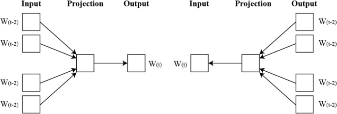
Representation of word2vec model (CBOW and Skip Gram).
Transfer learning using RoBERTa
Transfer learning with RoBERTa applies pre-trained language models to improve performance on specific NLP tasks by adapting previously learned knowledge. As depicted in Fig. 3, RoBERTa undergoes an initial pre-training phase on extensive corpora, allowing it to capture nuanced language patterns. This is followed by a fine-tuning phase tailored to particular tasks, where RoBERTa’s pre-trained representations are optimized for task-specific requirements. Multi-stage transfer learning strategy to better adapt the pre-trained RoBERTa model for fake news detection in limited-data scenarios. Initially, the model undergoes fine-tuning on a related large corpus to learn domain-specific features. Subsequently, a second fine-tuning phase is performed on the smaller target datasets (Politifact and GossipCop), with carefully controlled learning rates and layer freezing to prevent overfitting. This two-stage process allows the model to retain generalized language understanding while gradually specializing in the fake news detection task, improving accuracy and robustness compared to single-step fine-tuning approaches.

Architecture of RoBERTa model.
Token and positional embeddings
RoBERTa begins by transforming the input text sequence into a series of token embeddings. Each token \(x_i\) is mapped to a high-dimensional vector representation through a learnable embedding matrix. Specifically, for each input token \(x_i\), its corresponding embedding \(E(x_i)\) is calculated as:
$$\begin{aligned} E(x_i) = W_e \cdot x_i \end{aligned}$$
(8)
where \(x_i\) is a one-hot encoded representation of the token and \(W_e\) is an embedding matrix which is learnt through the training process. This transformation permits RoBERTa to connect discrete tokens to a continuous vector space, implying that the relations among words are accessible.
Moreover, since the transformer model does not capture the relative location of the tokens in a sequence, the positional encoding is added to the token vectors. These surrounding embeddings assist in keeping in touch with the location of the tokens and their significance within the sequence to assist towards the full comprehension of the input’s architecture in RoBERTa. The positional embedding for each of the tokens at position i is computed as follows:
$$\begin{aligned} P(x_i) = W_p \cdot i \end{aligned}$$
(9)
where \(W_p\) is a trainable embedding matrix, similar to token embeddings, and i is the token index within the sequence. In the final input representation \(H_0 (x_i)\) of each token \(x_i\), such as the position embedding, embedding for each token, embedding for each token, is associated with linear transformation.
$$\begin{aligned} H_0(x_i) = E(x_i) + P(x_i) \end{aligned}$$
(10)
Self-attention mechanism
RoBERTa consists of a multi-headed self-attention layer, which enables the model to evaluate the importance of each token to other tokens in the input sequence. For each token \(x_i\), three vectors are computed: query Q, key K, and value V, from the token’s input representation \(H_0 (x_i )\). These vectors are obtained through linear transformations using learnable matrices:
$$\begin{aligned} Q= & H_0(x_i) \cdot W_Q\end{aligned}$$
(11)
$$\begin{aligned} K= & H_0(x_i) \cdot W_K\end{aligned}$$
(12)
$$\begin{aligned} V= & H_0(x_i) \cdot W_V \end{aligned}$$
(13)
where \(W_Q\), \(W_K\), and \(W_V\) are learned projection matrices. The self-attention mechanism calculates the attention score between each token i and every other token j in the sequence by taking the dot product of the query and key vectors, followed by a scaling factor proportional to the square root of the dimensionality \(d_k\):
$$\begin{aligned} A_{ij} = \frac{Q_i \cdot K_j^\top }{\sqrt{d_k}} \end{aligned}$$
(14)
These attention scores indicate the level of significance that token i attributes to token j. In order to normalize the attention scores, a softmax function is utilized, which transforms the raw scores into a probability distribution:
$$\begin{aligned} a_{ij} = \text {softmax}(A_{ij}) = \frac{\exp (A_{ij})}{\sum _{j=1}^n \exp (A_{ij})} \end{aligned}$$
(15)
The weighted aggregate of all value vectors \(V_j\), where the weights are the normalized attention scores \(a_{ij}\), is the final output of the self-attention mechanism for token i.
$$\begin{aligned} O_i = \sum _{j=1}^n a_{ij} \cdot V_j \end{aligned}$$
(16)
Multi-head attention and layer normalization
RoBERTa employs multi-head attention to strengthen the model’s capabilities for capturing various contextual concepts encountered in the input sequence. In this form of attention, the self-attention technique is performed in parallel h number of times with each attention head having its distinct attention parameters. All the projection led outputs of attention heads concatenated and were minimal compression transformation through the projection matrix \(W_O\).
$$\begin{aligned} O_{\text {multi-head}} = \text {Concat}(O_1, O_2, \dots , O_h) \cdot W_O \end{aligned}$$
(17)
The multi-head attention mechanism enables the model to focus on multiple segments of the input sequence simultaneously, improving the understanding of each token in its context. RoBERTa further applies residual connections and layer normalizations after the multi-head attention layer to promote stability during the training process as well as convergence of the model. The output of the multi-head attention layer is also conveyed as input to the previous layer through a residual connection and thus the input is added to the layer output.
$$\begin{aligned} H_l(x_i) = \text {LayerNorm}\big (O_{\text {multi-head}}(x_i) + H_{l-1}(x_i)\big ) \end{aligned}$$
(18)
\(H_l(x_i)\) represent the output representation of token \(x_i\) after layer l.
Feed-forward neural network
Every layer of the RoBERTa contains a position wise feed forward neural network (FFN), which operates on each token independently. The FFN contains two linear layers separated by a ReLU. Token outputs are computed as follows:
$$\begin{aligned} \text {FFN}(x) = \max (0, x W_1 + b_1) W_2 + b_2 \end{aligned}$$
(19)
where \(W_1\) and \(W_2\) are the weight matrices, \(b_1\) and \(b_2\) are biases. In addition, the layer provides the model with non-linearity, improving the ability to process token representations.
Pre-training objective: masked language modelling (MLM)
RoBERTa is pre-trained with the masked language modelling (MLM) aim. In this setting, some of the tokens in the input sequence are retrieved at random, whereas the model must learn to predict what those hidden tokens are from the context provided by the other visible tokens. The loss function corresponding to the MLM is described as follows:
$$\begin{aligned} L_{\text {MLM}} = -\sum _{m=1}^M \log P(x_m \mid x_{\setminus m}) \end{aligned}$$
(20)
M represents the quantity of masked tokens, while \(P(x_{\setminus m})\) denotes the probability attributed to the accurate token \(x_m\), contingent upon the unmasked tokens in the sequence \((x_{\setminus m})\). This pre-training exercise enables RoBERTa to acquire profound contextual representations of words.
Fine tuning
Fine-tuning RoBERTa involves adapting a pre-trained language model for a specific task by updating its weights using a labeled dataset, allowing the model to capture task-specific patterns while leveraging its rich pre-trained knowledge. This process typically involves adding a task-specific output layer (e.g., a classification head) and optimizing the model end-to-end with a loss function, such as cross-entropy for classification tasks. The objective during fine-tuning can be expressed as minimizing the task-specific loss \(L(\theta )\) where \(\theta\) represents the model parameters being updated:
$$\begin{aligned} \theta ^* = \arg \min _{\theta } L(\theta ) \end{aligned}$$
(21)
Fine-tuning of RoBERTa was performed with a learning rate of 0.001 using the Adam optimizer and a batch size of 16. Early stopping based on validation loss was applied to avoid overfitting. We experimented with freezing initial transformer layers to evaluate the impact on model generalization, ultimately selecting the configuration yielding the best validation performance. Our methodology combines domain-tailored preprocessing, embedding technique evaluation, and a novel multi-stage transfer learning framework. This integrated design addresses the challenges of fake news detection on small datasets, leading to improved classification accuracy and robustness over conventional fine-tuning methods.
link


